Partitioning genetic trends in mean and variance

In breeding programmes, the observed genetic change is a sum of the contributions of different groups of individuals. Here we show how to partition the genetic mean and variance of breeding values using AlphaPart.

In addition to the contribution of paths to changes in genetic mean, breeding programmes should also consider analysing changes in genetic variance to understand the drivers of genetic change in a population fully. Managing the change in genetic mean and variance in breeding programmes is essential to ensure long-term genetic gain.

Loading packages

#=======================================================================
# Packges
#=======================================================================
#devtools::install_github("AlphaGenes/AlphaPart")
library(AlphaPart)
library(dplyr)
library(ggplot2)
library(ggridges)

Loading datafile

#=======================================================================
# Reading and organizing Scenario 1
#=======================================================================
data <-  readRDS("./../inst/extdata/AlphaPartCattleSim.rds") %>%
  dplyr::mutate(across(generation:mother, as.numeric)) %>%
  dplyr::rename(status = type) %>%
  dplyr::mutate(across(c("sex", "status"), as.factor)) %>%
  dplyr::mutate(path = interaction(sex,status, sep = ":")) %>%
  arrange(generation, ind) %>%
  select(ind, father, mother, sex, status, path, generation, tbv, pheno) %>%
  dplyr::mutate(generation = generation - 20) %>%
  droplevels()

# Data head
head(data) %>%
  knitr::kable(digits = 2)

ind	sex	status	path	generation	tbv	pheno
1	M	Non-Selected	M:Non-Selected	-20	-0.27	-0.48
2	F	Non-Selected	F:Non-Selected	-20	0.75	0.89
3	M	Non-Selected	M:Non-Selected	-20	-0.10	-0.04
4	F	Non-Selected	F:Non-Selected	-20	-0.53	-1.44
5	M	Non-Selected	M:Non-Selected	-20	0.70	0.88
6	F	Non-Selected	F:Non-Selected	-20	0.25	-0.63

# Data size
dim(data)

## [1] 42000     9

ind - individual
father and mother - individual’s parents
sex - individual sex
status - if the individual is or not selected
path - the path variable used to partition the additive genetic mean
tbv - true breeding value
pheno - phenotypic value

Partitioning trends in genetic mean and variance

We use the AlphaPart function to partition the true breeding values (tbv) in the data by the animal sex and status variable combination into females (F) and males (M) non-selected (N) and males selected (S) contributions:

part <- AlphaPart(data, colId = "ind", colFid = "father", 
                  colMid = "mother", colBV = "tbv", colPath = "path")

## 
## Size:
##  - individuals: 42000 
##  - traits: 1 (tbv)
##  - paths: 3 (F:Non-Selected, M:Non-Selected, M:Selected)
##  - unknown (missing) values:
## tbv 
##   0

head(part$tbv) %>%
  knitr::kable(digits = 2)

ind	sex	status	path	generation	pheno	tbv	tbv_w	tbv_F:Non-Selected	tbv_M:Non-Selected
1	M	Non-Selected	M:Non-Selected	-20	-0.48	-0.27	-0.27	0.00	-0.27
2	F	Non-Selected	F:Non-Selected	-20	0.89	0.75	0.75	0.75	0.00
3	M	Non-Selected	M:Non-Selected	-20	-0.04	-0.10	-0.10	0.00	-0.10
4	F	Non-Selected	F:Non-Selected	-20	-1.44	-0.53	-0.53	-0.53	0.00
5	M	Non-Selected	M:Non-Selected	-20	0.88	0.70	0.70	0.00	0.70
6	F	Non-Selected	F:Non-Selected	-20	-0.63	0.25	0.25	0.25	0.00

We use the generic summary.AlphaPart function to summarize an AlphaPart object by generation, con*sering:

the function mean

# Trends in the additve genetic mean
partMean <- summary(part, by = "generation", FUN = mean)

head(partMean$tbv) %>%
  knitr::kable(digits = 2)

generation	N	Sum	F:Non-Selected	M:Non-Selected	M:Selected
-20	2000	0.00	0.00	0.00	0.00
-19	1000	-0.12	0.00	0.00	-0.12
-18	1000	0.31	0.13	-0.01	0.18
-17	1000	0.68	0.17	0.00	0.51
-16	1000	1.14	0.34	0.01	0.79
-15	1000	1.34	0.37	0.00	0.97

the function variance

# Trends in the additive genetic variance
partVar <- summary(part, by = "generation", FUN = var, cov = TRUE)

head(partVar$tbv) %>%
  knitr::kable(digits = 2)

generation	N	Sum	F:Non-Selected	M:Non-Selected	M:Selected	F:Non-SelectedM:Non-Selected	F:Non-SelectedM:Selected	M:Non-SelectedM:Selected
-20	2000	0.30	0.15	0.15	0.00	0.00	0.00	0.00
-19	1000	0.31	0.15	0.07	0.08	0.00	0.00	0.00
-18	1000	0.24	0.16	0.06	0.05	0.00	-0.04	0.01
-17	1000	0.27	0.14	0.06	0.08	0.00	-0.01	0.00
-16	1000	0.19	0.11	0.06	0.03	0.00	-0.01	0.00
-15	1000	0.21	0.15	0.07	0.08	-0.01	-0.08	0.00

Example of plots to analyse the results

Distribution of breeding value partitions by sex and selection status (selected males (M(S)), non-selected males (M(N)), and females (F)) over generations.

part$tbv %>%
  ggplot(aes(y = as.factor(generation), `tbv_F:Non-Selected`)) +
  geom_density_ridges(
    aes(fill = "F - Non-Selected", linetype = "F - Non-Selected"),
    alpha = .4, point_alpha = 1, rel_min_height = 0.01
  ) +
  geom_density_ridges(
    aes(y = as.factor(generation), x= `tbv_M:Non-Selected`, fill = "M - Non-Selected",
        linetype = "M - Non-Selected"),
    alpha = .4, point_alpha = 1, rel_min_height = 0.01
  ) +
  geom_density_ridges(
    aes(y = as.factor(generation), x= `tbv_M:Selected`, fill = "M - Selected",
        linetype = "M - Selected"),
    alpha = .4, point_alpha = 1, rel_min_height = 0.01
  ) +
  geom_density_ridges(
    aes(y = as.factor(generation), x= `tbv`,
        fill = "Sum", linetype = "Sum"),
    alpha = .4, point_alpha = 1, rel_min_height = 0.01
  ) +
  ylab("Generation") +
  xlab("Density plot of breeding value partitions") +
  labs(fill = "Path:", linetype = "Path:") +
  theme_bw(base_size = 20) +
  theme(
    legend.position = "top"
  )

## Picking joint bandwidth of 0.0624

## Picking joint bandwidth of 0.0073

## Picking joint bandwidth of 0.0357

## Picking joint bandwidth of 0.0918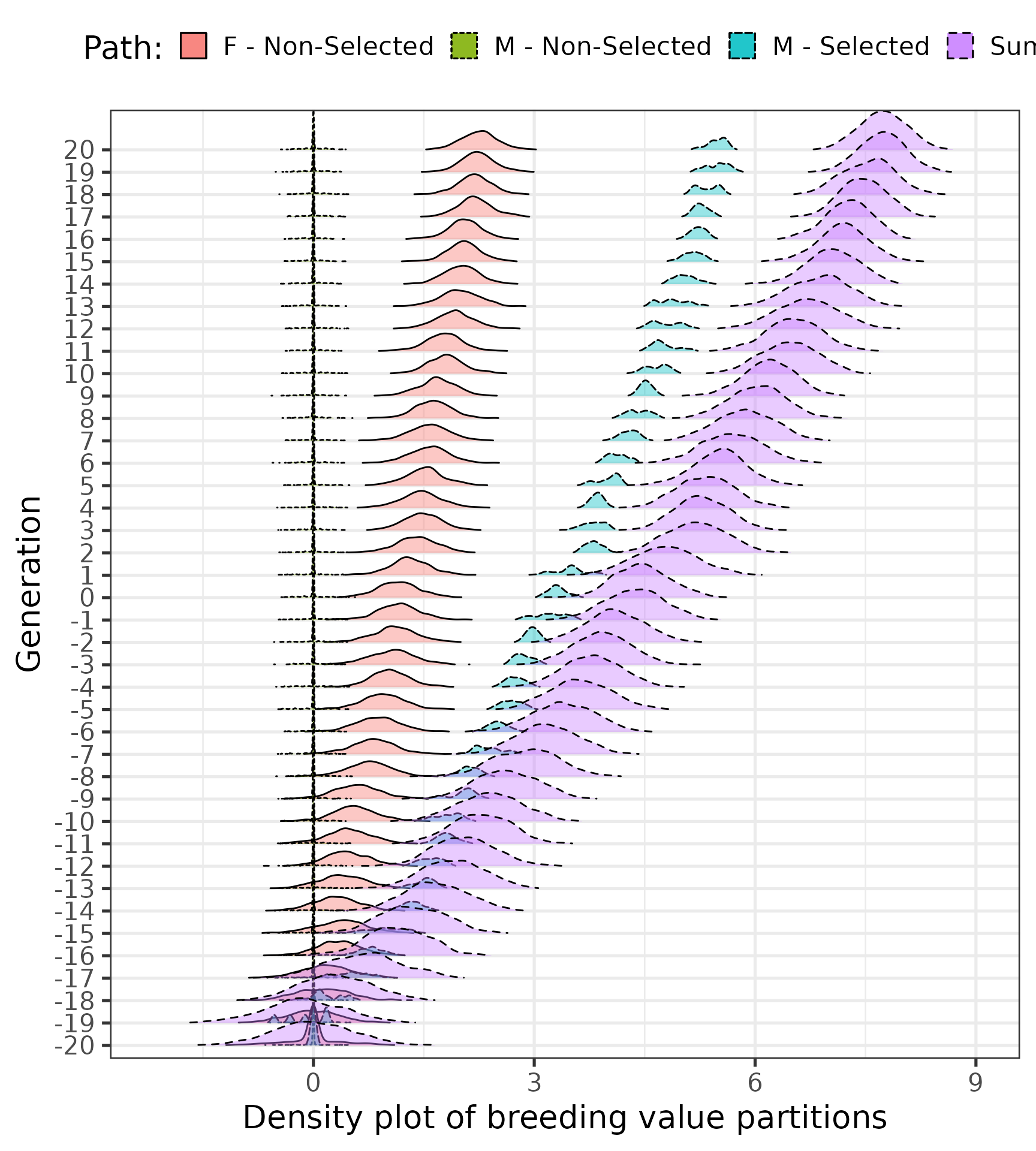

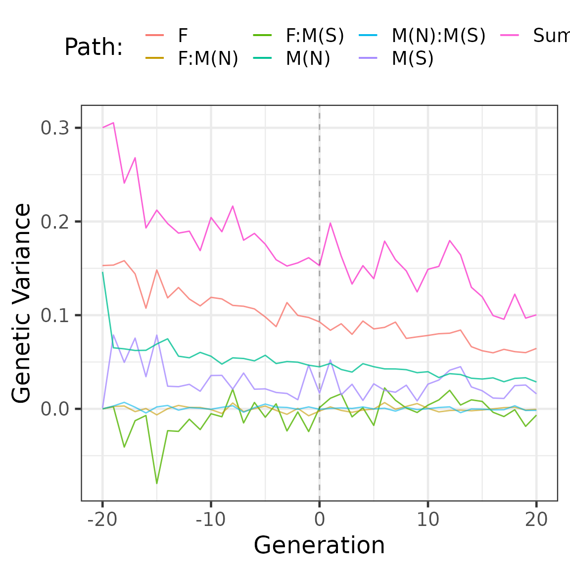
Partitions of genetic mean and variance by sex and selection status (selected males (M(S)), non-selected males (M(N)), and females (F)) using true breeding values:

partMean$tbv %>%
  ggplot(aes(y = Sum, x = generation, colour = "Sum"),
         size = 0.1) +
  scale_linetype_manual(
    values = c("solid", "longdash", "dashed", "dotted"))+
  geom_line() +
  geom_line(aes(y = `F:Non-Selected`, x = generation, 
                colour = "F"), alpha = 0.8) +
  geom_line(aes(y = `M:Selected`, x = generation,
                colour = "M(S)"), alpha = 0.8) +
  geom_line(aes(y = `M:Non-Selected`, x = generation,
                colour = "M(N)"), alpha = 0.8) +
  geom_vline(xintercept = 0, linetype = 2, alpha = 0.3) +
  ylab("Genetic Mean") +
  xlab("Generation") +
  labs(colour = "Path:") +
  theme_bw(base_size = 18) + 
  theme(legend.position = "top")

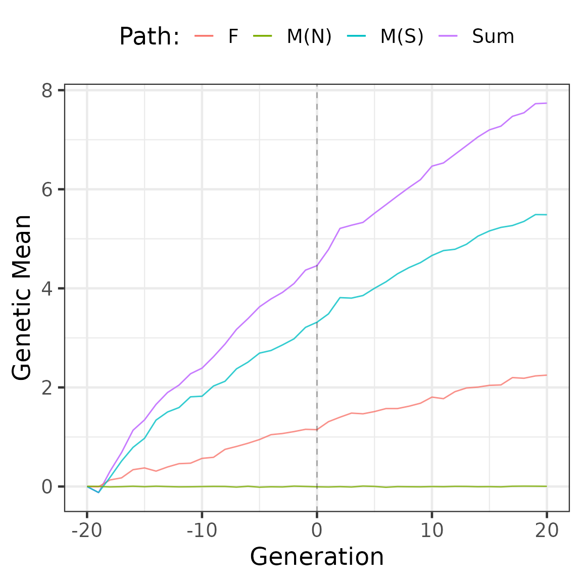
partVar$tbv %>%
  ggplot(aes(y = Sum, x = generation, colour = "Sum")) +
  geom_line() +
  geom_line(aes(y = `F:Non-Selected`, x = generation,
            colour = "F"), alpha = 0.8) +
  geom_line(aes(y = `F:Non-SelectedM:Selected`, x = generation,
            colour = "F:M(S)"), size =0.5, alpha =0.8) +
  geom_line(aes(y = `F:Non-SelectedM:Non-Selected`, x = generation,
            colour = "F:M(N)"), size =0.5, alpha =0.6) +
  geom_line(aes(y = `M:Non-SelectedM:Selected`, x = generation,
            colour = "M(N):M(S)"), size =0.5, alpha =0.6) +
  geom_line(aes(y = `M:Selected`, x = generation,
            colour = "M(S)"), alpha = 0.8) +
  geom_line(aes(y = `M:Non-Selected`, x = generation,
            colour = "M(N)"), size =0.5, alpha =0.8) +
  geom_vline(xintercept = 0, linetype = 2, alpha = 0.3) +
  ylab("Genetic Variance") +
  xlab("Generation") +
  labs(colour = "Path: ") +
  theme_bw(base_size = 18) +
  theme(
    legend.position = "top"
  )

## Warning: Using `size` aesthetic for lines was deprecated in ggplot2 3.4.0.
## ℹ Please use `linewidth` instead.
## This warning is displayed once every 8 hours.
## Call `lifecycle::last_lifecycle_warnings()` to see where this warning was
## generated.

Gregor Gorjanc, Jana Obsteter, Thiago de Paula Oliveira

2023-12-16

Loading packages

Loading datafile

Partitioning trends in genetic mean and variance

Example of plots to analyse the results