AlphaPart.R
AlphaPart.RdA function to partition breeding values by a path variable. The partition method is described in García-Cortés et al., 2008: Partition of the genetic trend to validate multiple selection decisions. Animal : an international journal of animal bioscience. DOI: doi:10.1017/S175173110800205X
Usage
AlphaPart(x, pathNA, recode, unknown, sort, verbose, profile,
  printProfile, pedType, colId, colFid, colMid, colPath, colBV,
  colBy, center, scaleEBV)
Arguments
- x
data.frame , with (at least) the following columns: individual, father, and mother identif ication, and year of birth; see arguments
colId,colFid,colMid,colPath, andcolBV; see also details about the validity of pedigree.- pathNA
Logical, set dummy path (to "XXX") where path information is unknown (missing).
- recode
Logical, internally recode individual, father and, mother identification to
1:ncodes, while missing parents are defined with0; this option must be used if identif ications inxare not already given as1:ncodes, see also argumentsort.- unknown
Value(s) used for representing unknown (missing) parent in
x; this options has an effect only whenrecode=FALSEas it is only needed in that situation.- sort
Logical, initially sort
xusingorderPed()so that children follow parents in order to make imputation as optimal as possible (imputation is performed within a loop from the first to the last unknown birth year); at the end original order is restored.- verbose
Numeric, print additional information:
0- print nothing,1- print some summaries about the data.- profile
Logical, collect timings and size of objects.
- printProfile
Character, print profile info on the fly (
"fly") or at the end ("end").- pedType
Character, pedigree type: the most common form is
"IPP"for Individual, Parent 1 (say father), and Parent 2 (say mother) data; the second form is"IPG"for Individual, Parent 1 (say father), and one of Grandparents of Parent 2 (say maternal grandfather).- colId
Numeric or character, position or name of a column holding individual identif ication.
- colFid
Numeric or character, position or name of a column holding father identif ication.
- colMid
Numeric or character, position or name of a column holding mother identif ication or maternal grandparent identif ication if
pedType="IPG".- colPath
Numeric or character, position or name of a column holding path information.
- colBV
Numeric or character, position(s) or name(s) of column(s) holding breeding Values.
- colBy
Numeric or character, position or name of a column holding group information (see details).
- center
Logical, if
center=TRUEdetect a shift in base population mean and attributes it as parent average effect rather than Mendelian sampling effect, otherwise, if center=FALSE, the base population values are only accounted as Mendelian sampling effect. Default iscenter = TRUE.- scaleEBV
a list with two arguments defining whether is appropriate to center and/or scale the
colBVcolumns in respect to the base population. The list may contain the following components:center: a logical valuescale: a logical value. Ifcenter = TRUEandscale = TRUEthen the base population is set to has zero mean and unit variance.
Value
An object of class AlphaPart, which can be used in
further analyses - there is a handy summary method
(summary.AlphaPart works on objects of
AlphaPart class) and a plot method for its output
(plot.summaryAlphaPart works on objects of
summaryAlphaPart class). Class AlphaPart is a
list. The first length(colBV) components (one for each trait
and named with trait label, say trt) are data frames. Each
data.frame contains:
xcolumns from initial dataxtrt_paparent averagetrt_wMendelian sampling termtrt_path1, trt_path2, ...breeding value partitions
The last component of returned object is also a list named
info with the following components holding meta information
about the analysis:
pathcolumn name holding path informationnPnumber of pathslPpath labelsnTnumber of traitslTtrait labelswarnpotential warning messages associated with this object
If colBy!=NULL the resulting object is of a class
summaryAlphaPart, see
summary.AlphaPart for details.
If profile=TRUE, profiling info is printed on screen to spot
any computational bottlenecks.
Details
Pedigree in x must be valid in a sense that there
are:
no directed loops (the simplest example is that the individual identification is equal to the identification of a father or mother)
no bisexuality, e.g., fathers most not appear as mothers
father and/or mother can be unknown (missing) - defined with any "code" that is different from existing identifications
Unknown (missing) values for breeding values are propagated down the
pedigree to provide all available values from genetic
evaluation. Another option is to cut pedigree links - set parents to
unknown and remove them from pedigree prior to using this function -
see pedSetBase function. Warning is issued
in the case of unknown (missing) values.
In animal breeding/genetics literature the model with the underlying
pedigree type "IPP" is often called animal model, while the
model for pedigree type "IPG" is often called sire - maternal
grandsire model. With a combination of colFid and
colMid mother - paternal grandsire model can be accomodated as
well.
Argument colBy can be used to directly perform a summary
analysis by group, i.e., summary(AlphaPart(...),
by="group"). See summary.AlphaPart for
more. This can save some CPU time by skipping intermediate
steps. However, only means can be obtained, while summary
method gives more flexibility.
References
Garcia-Cortes, L. A. et al. (2008) Partition of the genetic trend to validate multiple selection decisions. Animal, 2(6):821-824. doi:10.1017/S175173110800205X
See also
summary.AlphaPart for summary
method that works on output of AlphaPart,
pedSetBase for setting base population,
pedFixBirthYear for imputing unknown
(missing) birth years, orderPed in
pedigree package for sorting pedigree
Examples
## Small pedigree with additive genetic (=breeding) values
ped <- data.frame( id=c( 1, 2, 3, 4, 5, 6),
fid=c( 0, 0, 2, 0, 4, 0),
mid=c( 0, 0, 1, 0, 3, 3),
loc=c("A", "B", "A", "B", "A", "A"),
gen=c( 1, 1, 2, 2, 3, 3),
trt1=c(100, 120, 115, 130, 125, 125),
trt2=c(100, 110, 105, 100, 85, 110))
## Partition additive genetic values
tmp <- AlphaPart(x=ped, colBV=c("trt1", "trt2"))
#>
#> Size:
#> - individuals: 6
#> - traits: 2 (trt1, trt2)
#> - paths: 2 (A, B)
#> - unknown (missing) values:
#> trt1 trt2
#> 0 0
print(tmp)
#>
#>
#> Partitions of breeding values
#> - individuals: 6
#> - paths: 2 (A, B)
#> - traits: 2 (trt1, trt2)
#>
#> Trait: trt1
#>
#> id fid mid loc gen trt1 trt1_pa trt1_w trt1_A trt1_B
#> 1 1 0 0 A 1 100 116.6667 -16.666667 100 0
#> 2 2 0 0 B 1 120 116.6667 3.333333 0 120
#> 3 3 2 1 A 2 115 110.0000 5.000000 55 60
#> 4 4 0 0 B 2 130 116.6667 13.333333 0 130
#> 5 5 4 3 A 3 125 122.5000 2.500000 30 95
#> 6 6 0 3 A 3 125 57.5000 67.500000 95 30
#>
#> Trait: trt2
#>
#> id fid mid loc gen trt2 trt2_pa trt2_w trt2_A trt2_B
#> 1 1 0 0 A 1 100 103.3333 -3.333333 100.0 0.0
#> 2 2 0 0 B 1 110 103.3333 6.666667 0.0 110.0
#> 3 3 2 1 A 2 105 105.0000 0.000000 50.0 55.0
#> 4 4 0 0 B 2 100 103.3333 -3.333333 0.0 100.0
#> 5 5 4 3 A 3 85 102.5000 -17.500000 7.5 77.5
#> 6 6 0 3 A 3 110 52.5000 57.500000 82.5 27.5
#>
## Summarize by generation (genetic mean)
summary(tmp, by="gen")
#>
#>
#> Summary of partitions of breeding values
#> - paths: 2 (A, B)
#> - traits: 2 (trt1, trt2)
#>
#> Trait: trt1
#>
#> gen N Sum A B
#> 1 1 2 110.0 50.0 60.0
#> 2 2 2 122.5 27.5 95.0
#> 3 3 2 125.0 62.5 62.5
#>
#> Trait: trt2
#>
#> gen N Sum A B
#> 1 1 2 105.0 50 55.0
#> 2 2 2 102.5 25 77.5
#> 3 3 2 97.5 45 52.5
#>
## Summarize by generation (genetic variance)
summary(tmp, by="gen", FUN = var)
#>
#>
#> Summary of partitions of breeding values
#> - paths: 2 (A, B, Sum.Cov)
#> - traits: 2 (trt1, trt2)
#>
#> Trait: trt1
#>
#> gen N Sum A B Sum.Cov
#> 1 1 2 200.0 5000.0 7200.0 -12000
#> 2 2 2 112.5 1512.5 2450.0 -3850
#> 3 3 2 0.0 2112.5 2112.5 -4225
#>
#> Trait: trt2
#>
#> gen N Sum A B Sum.Cov
#> 1 1 2 50.0 5000.0 6050.0 -11000
#> 2 2 2 12.5 1250.0 1012.5 -2250
#> 3 3 2 312.5 2812.5 1250.0 -3750
#>
# \donttest{
## There are also two demos
demo(topic="AlphaPart_deterministic", package="AlphaPart",
ask=interactive())
#>
#>
#> demo(AlphaPart_deterministic)
#> ---- ~~~~~~~~~~~~~~~~~~~~~~~
#>
#> > ### partAGV_deterministic.R
#> > ###-----------------------------------------------------------------------------
#> > ### $Id$
#> > ###-----------------------------------------------------------------------------
#> >
#> > ### DESCRIPTION OF A DEMONSTRATION
#> > ###-----------------------------------------------------------------------------
#> >
#> > ## A demonstration with a simple example to see in action the partitioning of
#> > ## additive genetic values by paths (Garcia-Cortes et al., 2008; Animal)
#> > ##
#> > ## DETERMINISTIC SIMULATION (sort of)
#> > ##
#> > ## We have two locations (1 and 2). The first location has individualss with higher
#> > ## additive genetic value. Males from the first location are imported males to the
#> > ## second location from generation 2/3. This clearly leads to genetic gain in the
#> > ## second location. However, the second location can also perform their own selection
#> > ## so the question is how much genetic gain is due to the import of genes from the
#> > ## first location and due to their own selection.
#> > ##
#> > ## Above scenario will be tested with a simple example of a pedigree bellow. Two
#> > ## scenarios will be evaluated: without or with own selection in the second location.
#> > ## Selection will always be present in the first location.
#> > ##
#> > ## Additive genetic values are provided, i.e., no inference is being done!
#> > ##
#> > ## The idea of this example is not to do extensive simulations, but just to have
#> > ## a simple example to see how the partitioning of additive genetic values works.
#> >
#> > ### SETUP
#> > ###-----------------------------------------------------------------------------
#> >
#> > options(width=200)
#>
#> > ### EXAMPLE PEDIGREE & SETUP OF MENDELIAN SAMPLING - "DETERMINISTIC"
#> > ###-----------------------------------------------------------------------------
#> >
#> > ## Generation 0
#> > id0 <- c("01", "02", "03", "04")
#>
#> > fid0 <- mid0 <- rep(NA, times=length(id0))
#>
#> > h0 <- rep(c(1, 2), each=2)
#>
#> > g0 <- rep(0, times=length(id0))
#>
#> > w10 <- c( 2, 2, 0, 0)
#>
#> > w20 <- c( 2, 2, 0, 0)
#>
#> > ## Generation 1
#> > id1 <- c("11", "12", "13", "14")
#>
#> > fid1 <- c("01", "01", "03", "03")
#>
#> > mid1 <- c("02", "02", "04", "04")
#>
#> > h1 <- h0
#>
#> > g1 <- rep(1, times=length(id1))
#>
#> > w11 <- c( 0.6, 0.2, -0.6, 0.2)
#>
#> > w21 <- c( 0.6, 0.2, 0.6, 0.2)
#>
#> > ## Generation 2
#> > id2 <- c("21", "22", "23", "24")
#>
#> > fid2 <- c("12", "12", "12", "12")
#>
#> > mid2 <- c("11", "11", "13", "14")
#>
#> > h2 <- h0
#>
#> > g2 <- rep(2, times=length(id2))
#>
#> > w12 <- c( 0.6, 0.3, -0.2, 0.2)
#>
#> > w22 <- c( 0.6, 0.3, 0.2, 0.2)
#>
#> > ## Generation 3
#> > id3 <- c("31", "32", "33", "34")
#>
#> > fid3 <- c("22", "22", "22", "22")
#>
#> > mid3 <- c("21", "21", "23", "24")
#>
#> > h3 <- h0
#>
#> > g3 <- rep(3, times=length(id3))
#>
#> > w13 <- c( 0.7, 0.1, -0.3, 0.3)
#>
#> > w23 <- c( 0.7, 0.1, 0.3, 0.3)
#>
#> > ## Generation 4
#> > id4 <- c("41", "42", "43", "44")
#>
#> > fid4 <- c("32", "32", "32", "32")
#>
#> > mid4 <- c("31", "31", "33", "34")
#>
#> > h4 <- h0
#>
#> > g4 <- rep(4, times=length(id4))
#>
#> > w14 <- c( 0.8, 0.8, -0.1, 0.3)
#>
#> > w24 <- c( 0.8, 0.8, 0.1, 0.3)
#>
#> > ## Generation 5
#> > id5 <- c("51", "52", "53", "54")
#>
#> > fid5 <- c("42", "42", "42", "42")
#>
#> > mid5 <- c("41", "41", "43", "44")
#>
#> > h5 <- h0
#>
#> > g5 <- rep(5, times=length(id4))
#>
#> > w15 <- c( 0.8, 1.0, -0.2, 0.3)
#>
#> > w25 <- c( 0.8, 1.0, 0.2, 0.3)
#>
#> > ped <- data.frame( id=c( id0, id1, id2, id3, id4, id5),
#> + fid=c(fid0, fid1, fid2, fid3, fid4, fid5),
#> + mid=c(mid0, mid1, mid2, mid3, mid4, mid5),
#> + loc=c( h0, h1, h2, h3, h4, h5),
#> + gen=c( g0, g1, g2, g3, g4, g5),
#> + w1=c( w10, w11, w12, w13, w14, w15),
#> + w2=c( w20, w21, w22, w23, w24, w25))
#>
#> > ped$sex <- 2
#>
#> > ped[ped$id %in% ped$fid, "sex"] <- 1
#>
#> > ped$loc.gen <- with(ped, paste(loc, gen, sep="-"))
#>
#> > ### SIMULATE ADDITIVE GENETIC VALUES - SUM PARENT AVERAGE AND MENDELIAN SAMPLING
#> > ###-----------------------------------------------------------------------------
#> >
#> > ## Additive genetic mean in founders by location
#> > mu1 <- 2
#>
#> > mu2 <- 0
#>
#> > ## Additive genetic variance in population
#> > sigma2 <- 1
#>
#> > sigma <- sqrt(sigma2)
#>
#> > ## Threshold value for Mendelian sampling for selection - only values above this
#> > ## will be accepted in simulation
#> > t <- 0
#>
#> > ped$agv1 <- ped$pa1 <- NA ## Scenario (trait) 1: No selection in the second location
#>
#> > ped$agv2 <- ped$pa2 <- NA ## Scenario (trait) 2: Selection in the second location
#>
#> > ## Generation 0 - founders (no parent average here - so setting it to zero)
#> > ped[ped$gen == 0, c("pa1", "pa2")] <- 0
#>
#> > ped[ped$gen == 0, c("agv1", "agv2")] <- ped[ped$gen == 0, c("w1", "w2")]
#>
#> > ## Generation 1+ - non-founders (parent average + Mendelian sampling)
#> > for(i in (length(g0)+1):nrow(ped)) {
#> + ped[i, "pa1"] <- 0.5 * (ped[ped$id %in% ped[i, "fid"], "agv1"] +
#> + ped[ped$id %in% ped[i, "mid"], "agv1"])
#> + ped[i, "pa2"] <- 0.5 * (ped[ped$id %in% ped[i, "fid"], "agv2"] +
#> + ped[ped$id %in% ped[i, "mid"], "agv2"])
#> + ped[i, c("agv1", "agv2")] <- ped[i, c("pa1", "pa2")] + ped[i, c("w1", "w2")]
#> + }
#>
#> > ### PLOT INDIVIDUAL ADDITIVE GENETIC VALUES
#> > ###-----------------------------------------------------------------------------
#> >
#> > par(mfrow=c(2, 1), bty="l", pty="m", mar=c(2, 2, 1, 1) + .1, mgp=c(0.7, 0.2, 0))
#>
#> > tmp <- ped$gen + c(-1.5, -0.5, 0.5, 1.5) * 0.1
#>
#> > with(ped, plot(agv1 ~ tmp, pch=c(19, 21)[ped$loc], ylab="Additive genetic value",
#> + xlab="Generation", main="Selection in location 1", axes=FALSE,
#> + ylim=range(c(agv1, agv2))))
#>
#> > axis(1, labels=FALSE, tick=FALSE); axis(2, labels=FALSE, tick=FALSE); box()
#>
#> > legend(x="topleft", legend=c(1, 2), title="Location", pch=c(19, 21), bty="n")
#>
#> > with(ped, plot(agv2 ~ tmp, pch=c(19, 21)[ped$loc], ylab="Additive genetic value",
#> + xlab="Generation", main="Selection in locations 1 and 2", axes=FALSE,
#> + ylim=range(c(agv1, agv2))))
 #>
#> > axis(1, labels=FALSE, tick=FALSE); axis(2, labels=FALSE, tick=FALSE); box()
#>
#> > legend(x="topleft", legend=c(1, 2), title="Location", pch=c(19, 21), bty="n")
#>
#> > ### PARTITION ADDITIVE GENETIC VALUES BY ...
#> > ###-----------------------------------------------------------------------------
#> >
#> > ## Compute partitions by location
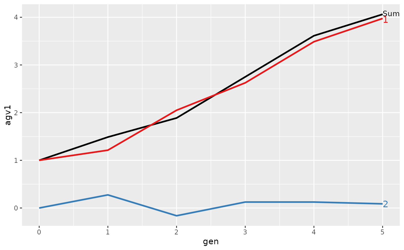
#> > (res <- AlphaPart(x=ped, colPath="loc", colBV=c("agv1", "agv2")))
#>
#> Size:
#> - individuals: 24
#> - traits: 2 (agv1, agv2)
#> - paths: 2 (1, 2)
#> - unknown (missing) values:
#> agv1 agv2
#> 0 0
#>
#>
#> Partitions of breeding values
#> - individuals: 24
#> - paths: 2 (1, 2)
#> - traits: 2 (agv1, agv2)
#>
#> Trait: agv1
#>
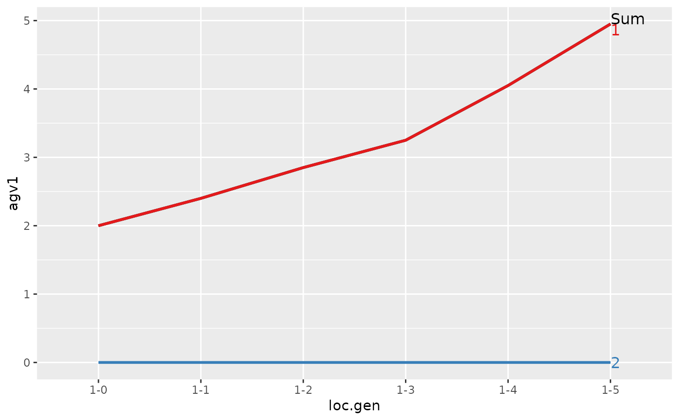
#> id fid mid loc gen w1 w2 sex loc.gen pa1 pa2 agv1 agv1_pa agv1_w agv1_1 agv1_2
#> 1 01 <NA> <NA> 1 0 2.0 2.0 1 1-0 0 0 2.0 0 2.0 2.0 0
#> 2 02 <NA> <NA> 1 0 2.0 2.0 2 1-0 0 0 2.0 0 2.0 2.0 0
#> 3 03 <NA> <NA> 2 0 0.0 0.0 1 2-0 0 0 0.0 0 0.0 0.0 0
#> 4 04 <NA> <NA> 2 0 0.0 0.0 2 2-0 0 0 0.0 0 0.0 0.0 0
#> 5 11 01 02 1 1 0.6 0.6 2 1-1 2 2 2.6 2 0.6 2.6 0
#> 6 12 01 02 1 1 0.2 0.2 1 1-1 2 2 2.2 2 0.2 2.2 0
#> ...
#> id fid mid loc gen w1 w2 sex loc.gen pa1 pa2 agv1 agv1_pa agv1_w agv1_1 agv1_2
#> 19 43 32 33 2 4 -0.1 0.1 2 2-4 2.15 2.700 2.05 2.15 -0.1 2.4250 -0.3750
#> 20 44 32 34 2 4 0.3 0.3 2 2-4 2.65 2.650 2.95 2.65 0.3 2.4250 0.5250
#> 21 51 42 41 1 5 0.8 0.8 2 1-5 4.05 4.050 4.85 4.05 0.8 4.8500 0.0000
#> 22 52 42 41 1 5 1.0 1.0 2 1-5 4.05 4.050 5.05 4.05 1.0 5.0500 0.0000
#> 23 53 42 43 2 5 -0.2 0.2 2 2-5 3.05 3.425 2.85 3.05 -0.2 3.2375 -0.3875
#> 24 54 42 44 2 5 0.3 0.3 2 2-5 3.50 3.500 3.80 3.50 0.3 3.2375 0.5625
#>
#> Trait: agv2
#>
#> id fid mid loc gen w1 w2 sex loc.gen pa1 pa2 agv2 agv2_pa agv2_w agv2_1 agv2_2
#> 1 01 <NA> <NA> 1 0 2.0 2.0 1 1-0 0 0 2.0 0 2.0 2.0 0
#> 2 02 <NA> <NA> 1 0 2.0 2.0 2 1-0 0 0 2.0 0 2.0 2.0 0
#> 3 03 <NA> <NA> 2 0 0.0 0.0 1 2-0 0 0 0.0 0 0.0 0.0 0
#> 4 04 <NA> <NA> 2 0 0.0 0.0 2 2-0 0 0 0.0 0 0.0 0.0 0
#> 5 11 01 02 1 1 0.6 0.6 2 1-1 2 2 2.6 2 0.6 2.6 0
#> 6 12 01 02 1 1 0.2 0.2 1 1-1 2 2 2.2 2 0.2 2.2 0
#> ...
#> id fid mid loc gen w1 w2 sex loc.gen pa1 pa2 agv2 agv2_pa agv2_w agv2_1 agv2_2
#> 19 43 32 33 2 4 -0.1 0.1 2 2-4 2.15 2.700 2.800 2.700 0.1 2.4250 0.3750
#> 20 44 32 34 2 4 0.3 0.3 2 2-4 2.65 2.650 2.950 2.650 0.3 2.4250 0.5250
#> 21 51 42 41 1 5 0.8 0.8 2 1-5 4.05 4.050 4.850 4.050 0.8 4.8500 0.0000
#> 22 52 42 41 1 5 1.0 1.0 2 1-5 4.05 4.050 5.050 4.050 1.0 5.0500 0.0000
#> 23 53 42 43 2 5 -0.2 0.2 2 2-5 3.05 3.425 3.625 3.425 0.2 3.2375 0.3875
#> 24 54 42 44 2 5 0.3 0.3 2 2-5 3.50 3.500 3.800 3.500 0.3 3.2375 0.5625
#>
#>
#> > ## Summarize whole population
#> > (ret <- summary(res))
#>
#>
#> Summary of partitions of breeding values
#> - paths: 2 (1, 2)
#> - traits: 2 (agv1, agv2)
#>
#> Trait: agv1
#>
#> N <NA> Sum 1 2
#> 1 1 24 2.33125 2.346875 -0.015625
#>
#> Trait: agv2
#>
#> N <NA> Sum 1 2
#> 1 1 24 2.532292 2.346875 0.1854167
#>
#>
#> > ## Summarize and plot by generation (=trend)
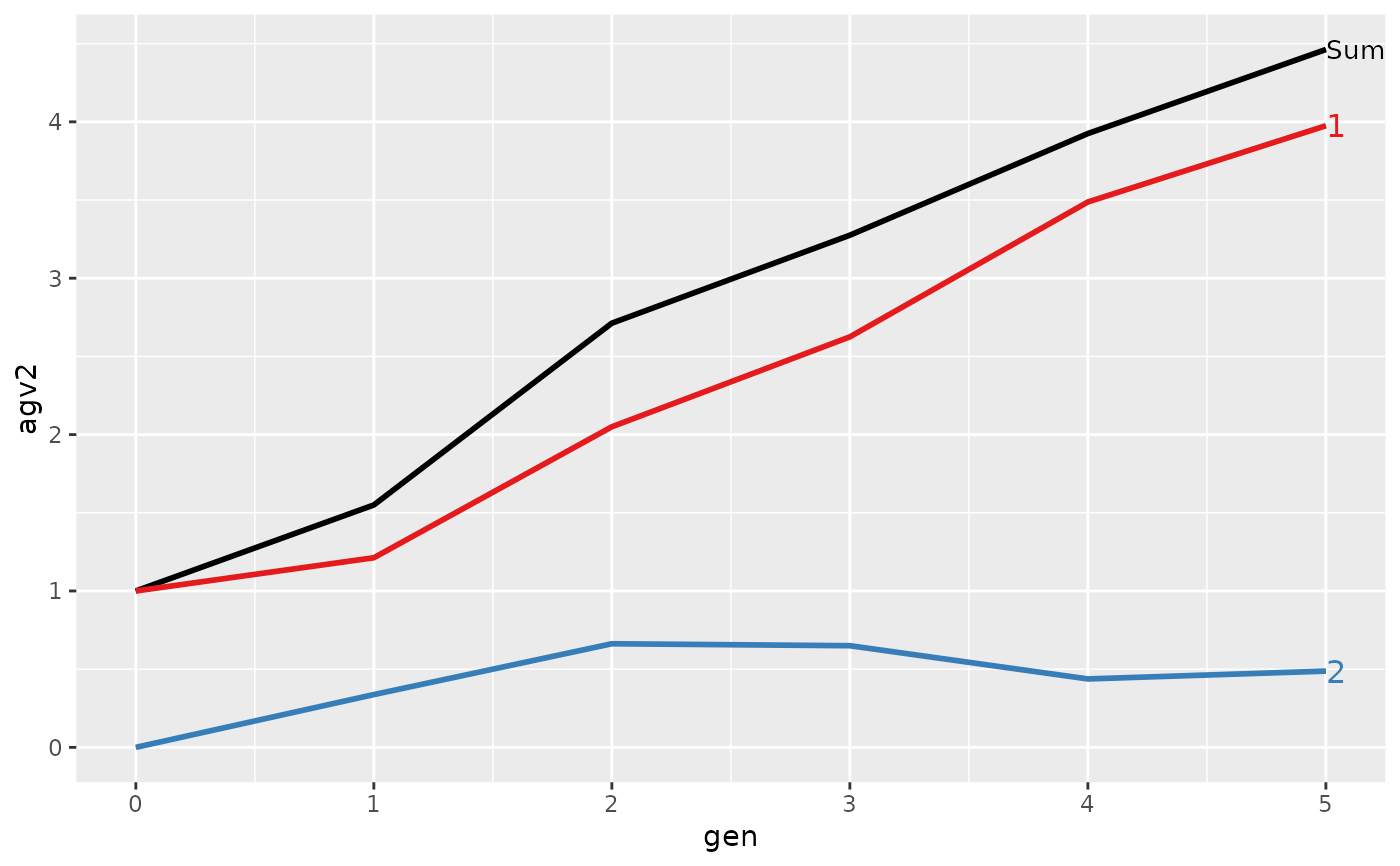
#> > (ret <- summary(res, by="gen"))
#>
#>
#> Summary of partitions of breeding values
#> - paths: 2 (1, 2)
#> - traits: 2 (agv1, agv2)
#>
#> Trait: agv1
#>
#> gen N Sum 1 2
#> 1 0 4 1.0000 1.00000 0.00000
#> 2 1 4 1.1000 1.20000 -0.10000
#> 3 2 4 1.9250 1.97500 -0.05000
#> 4 3 4 2.5500 2.57500 -0.02500
#> 5 4 4 3.2750 3.23750 0.03750
#> 6 5 4 4.1375 4.09375 0.04375
#>
#> Trait: agv2
#>
#> gen N Sum 1 2
#> 1 0 4 1.00000 1.00000 0.0000
#> 2 1 4 1.40000 1.20000 0.2000
#> 3 2 4 2.17500 1.97500 0.2000
#> 4 3 4 2.82500 2.57500 0.2500
#> 5 4 4 3.46250 3.23750 0.2250
#> 6 5 4 4.33125 4.09375 0.2375
#>
#>
#> > plot(ret)
#> Warning: `qplot()` was deprecated in ggplot2 3.4.0.
#> ℹ The deprecated feature was likely used in the AlphaPart package.
#> Please report the issue to the authors.
#> Warning: Using `size` aesthetic for lines was deprecated in ggplot2 3.4.0.
#> ℹ Please use `linewidth` instead.
#> ℹ The deprecated feature was likely used in the AlphaPart package.
#> Please report the issue to the authors.
#> Warning: `aes_string()` was deprecated in ggplot2 3.0.0.
#> ℹ Please use tidy evaluation idioms with `aes()`.
#> ℹ See also `vignette("ggplot2-in-packages")` for more information.
#> ℹ The deprecated feature was likely used in the directlabels package.
#> Please report the issue at <https://github.com/tdhock/directlabels/issues>.
#>
#> > axis(1, labels=FALSE, tick=FALSE); axis(2, labels=FALSE, tick=FALSE); box()
#>
#> > legend(x="topleft", legend=c(1, 2), title="Location", pch=c(19, 21), bty="n")
#>
#> > ### PARTITION ADDITIVE GENETIC VALUES BY ...
#> > ###-----------------------------------------------------------------------------
#> >
#> > ## Compute partitions by location
#> > (res <- AlphaPart(x=ped, colPath="loc", colBV=c("agv1", "agv2")))
#>
#> Size:
#> - individuals: 24
#> - traits: 2 (agv1, agv2)
#> - paths: 2 (1, 2)
#> - unknown (missing) values:
#> agv1 agv2
#> 0 0
#>
#>
#> Partitions of breeding values
#> - individuals: 24
#> - paths: 2 (1, 2)
#> - traits: 2 (agv1, agv2)
#>
#> Trait: agv1
#>
#> id fid mid loc gen w1 w2 sex loc.gen pa1 pa2 agv1 agv1_pa agv1_w agv1_1 agv1_2
#> 1 01 <NA> <NA> 1 0 2.0 2.0 1 1-0 0 0 2.0 0 2.0 2.0 0
#> 2 02 <NA> <NA> 1 0 2.0 2.0 2 1-0 0 0 2.0 0 2.0 2.0 0
#> 3 03 <NA> <NA> 2 0 0.0 0.0 1 2-0 0 0 0.0 0 0.0 0.0 0
#> 4 04 <NA> <NA> 2 0 0.0 0.0 2 2-0 0 0 0.0 0 0.0 0.0 0
#> 5 11 01 02 1 1 0.6 0.6 2 1-1 2 2 2.6 2 0.6 2.6 0
#> 6 12 01 02 1 1 0.2 0.2 1 1-1 2 2 2.2 2 0.2 2.2 0
#> ...
#> id fid mid loc gen w1 w2 sex loc.gen pa1 pa2 agv1 agv1_pa agv1_w agv1_1 agv1_2
#> 19 43 32 33 2 4 -0.1 0.1 2 2-4 2.15 2.700 2.05 2.15 -0.1 2.4250 -0.3750
#> 20 44 32 34 2 4 0.3 0.3 2 2-4 2.65 2.650 2.95 2.65 0.3 2.4250 0.5250
#> 21 51 42 41 1 5 0.8 0.8 2 1-5 4.05 4.050 4.85 4.05 0.8 4.8500 0.0000
#> 22 52 42 41 1 5 1.0 1.0 2 1-5 4.05 4.050 5.05 4.05 1.0 5.0500 0.0000
#> 23 53 42 43 2 5 -0.2 0.2 2 2-5 3.05 3.425 2.85 3.05 -0.2 3.2375 -0.3875
#> 24 54 42 44 2 5 0.3 0.3 2 2-5 3.50 3.500 3.80 3.50 0.3 3.2375 0.5625
#>
#> Trait: agv2
#>
#> id fid mid loc gen w1 w2 sex loc.gen pa1 pa2 agv2 agv2_pa agv2_w agv2_1 agv2_2
#> 1 01 <NA> <NA> 1 0 2.0 2.0 1 1-0 0 0 2.0 0 2.0 2.0 0
#> 2 02 <NA> <NA> 1 0 2.0 2.0 2 1-0 0 0 2.0 0 2.0 2.0 0
#> 3 03 <NA> <NA> 2 0 0.0 0.0 1 2-0 0 0 0.0 0 0.0 0.0 0
#> 4 04 <NA> <NA> 2 0 0.0 0.0 2 2-0 0 0 0.0 0 0.0 0.0 0
#> 5 11 01 02 1 1 0.6 0.6 2 1-1 2 2 2.6 2 0.6 2.6 0
#> 6 12 01 02 1 1 0.2 0.2 1 1-1 2 2 2.2 2 0.2 2.2 0
#> ...
#> id fid mid loc gen w1 w2 sex loc.gen pa1 pa2 agv2 agv2_pa agv2_w agv2_1 agv2_2
#> 19 43 32 33 2 4 -0.1 0.1 2 2-4 2.15 2.700 2.800 2.700 0.1 2.4250 0.3750
#> 20 44 32 34 2 4 0.3 0.3 2 2-4 2.65 2.650 2.950 2.650 0.3 2.4250 0.5250
#> 21 51 42 41 1 5 0.8 0.8 2 1-5 4.05 4.050 4.850 4.050 0.8 4.8500 0.0000
#> 22 52 42 41 1 5 1.0 1.0 2 1-5 4.05 4.050 5.050 4.050 1.0 5.0500 0.0000
#> 23 53 42 43 2 5 -0.2 0.2 2 2-5 3.05 3.425 3.625 3.425 0.2 3.2375 0.3875
#> 24 54 42 44 2 5 0.3 0.3 2 2-5 3.50 3.500 3.800 3.500 0.3 3.2375 0.5625
#>
#>
#> > ## Summarize whole population
#> > (ret <- summary(res))
#>
#>
#> Summary of partitions of breeding values
#> - paths: 2 (1, 2)
#> - traits: 2 (agv1, agv2)
#>
#> Trait: agv1
#>
#> N <NA> Sum 1 2
#> 1 1 24 2.33125 2.346875 -0.015625
#>
#> Trait: agv2
#>
#> N <NA> Sum 1 2
#> 1 1 24 2.532292 2.346875 0.1854167
#>
#>
#> > ## Summarize and plot by generation (=trend)
#> > (ret <- summary(res, by="gen"))
#>
#>
#> Summary of partitions of breeding values
#> - paths: 2 (1, 2)
#> - traits: 2 (agv1, agv2)
#>
#> Trait: agv1
#>
#> gen N Sum 1 2
#> 1 0 4 1.0000 1.00000 0.00000
#> 2 1 4 1.1000 1.20000 -0.10000
#> 3 2 4 1.9250 1.97500 -0.05000
#> 4 3 4 2.5500 2.57500 -0.02500
#> 5 4 4 3.2750 3.23750 0.03750
#> 6 5 4 4.1375 4.09375 0.04375
#>
#> Trait: agv2
#>
#> gen N Sum 1 2
#> 1 0 4 1.00000 1.00000 0.0000
#> 2 1 4 1.40000 1.20000 0.2000
#> 3 2 4 2.17500 1.97500 0.2000
#> 4 3 4 2.82500 2.57500 0.2500
#> 5 4 4 3.46250 3.23750 0.2250
#> 6 5 4 4.33125 4.09375 0.2375
#>
#>
#> > plot(ret)
#> Warning: `qplot()` was deprecated in ggplot2 3.4.0.
#> ℹ The deprecated feature was likely used in the AlphaPart package.
#> Please report the issue to the authors.
#> Warning: Using `size` aesthetic for lines was deprecated in ggplot2 3.4.0.
#> ℹ Please use `linewidth` instead.
#> ℹ The deprecated feature was likely used in the AlphaPart package.
#> Please report the issue to the authors.
#> Warning: `aes_string()` was deprecated in ggplot2 3.0.0.
#> ℹ Please use tidy evaluation idioms with `aes()`.
#> ℹ See also `vignette("ggplot2-in-packages")` for more information.
#> ℹ The deprecated feature was likely used in the directlabels package.
#> Please report the issue at <https://github.com/tdhock/directlabels/issues>.
 #>
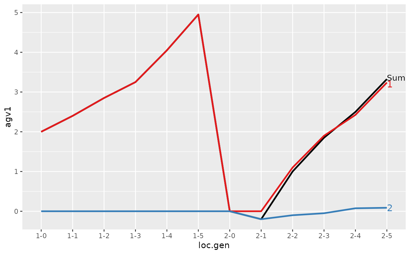
#> > ## Summarize and plot location specific trends
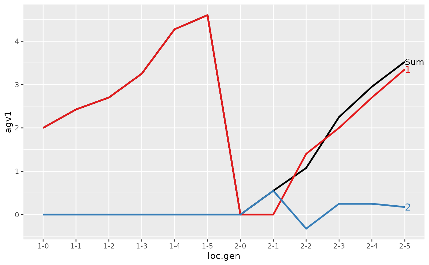
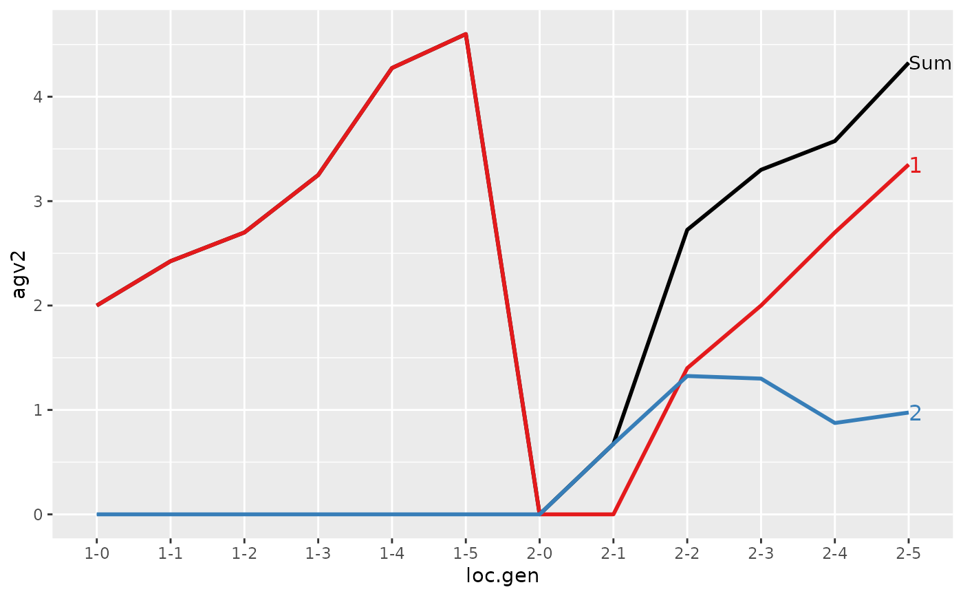
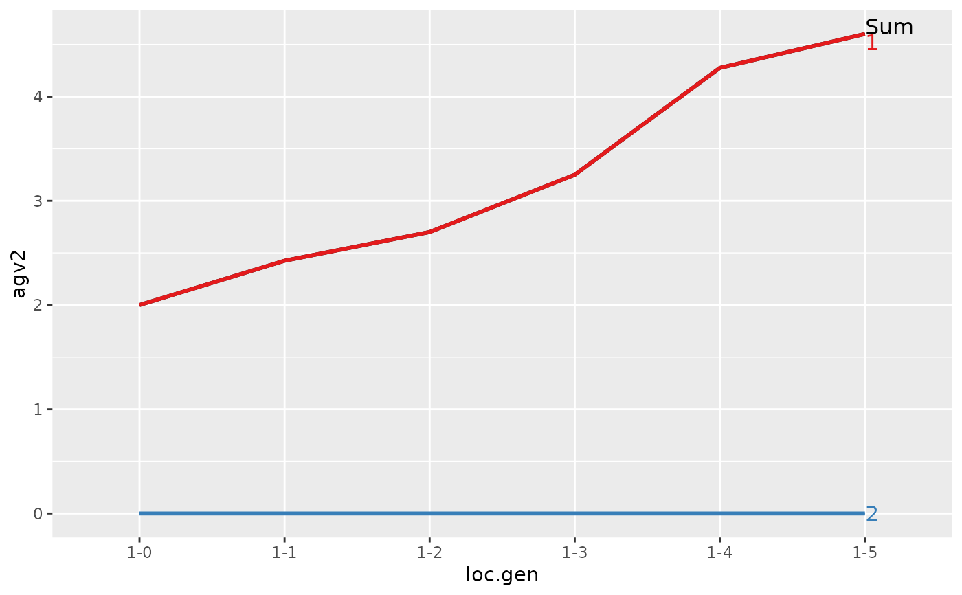
#> > (ret <- summary(res, by="loc.gen"))
#>
#>
#> Summary of partitions of breeding values
#> - paths: 2 (1, 2)
#> - traits: 2 (agv1, agv2)
#>
#> Trait: agv1
#>
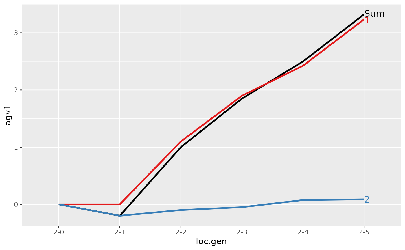
#> loc.gen N Sum 1 2
#> 1 1-0 2 2.000 2.0000 0.0000
#> 2 1-1 2 2.400 2.4000 0.0000
#> 3 1-2 2 2.850 2.8500 0.0000
#> 4 1-3 2 3.250 3.2500 0.0000
#> 5 1-4 2 4.050 4.0500 0.0000
#> 6 1-5 2 4.950 4.9500 0.0000
#> 7 2-0 2 0.000 0.0000 0.0000
#> 8 2-1 2 -0.200 0.0000 -0.2000
#> 9 2-2 2 1.000 1.1000 -0.1000
#> 10 2-3 2 1.850 1.9000 -0.0500
#> 11 2-4 2 2.500 2.4250 0.0750
#> 12 2-5 2 3.325 3.2375 0.0875
#>
#> Trait: agv2
#>
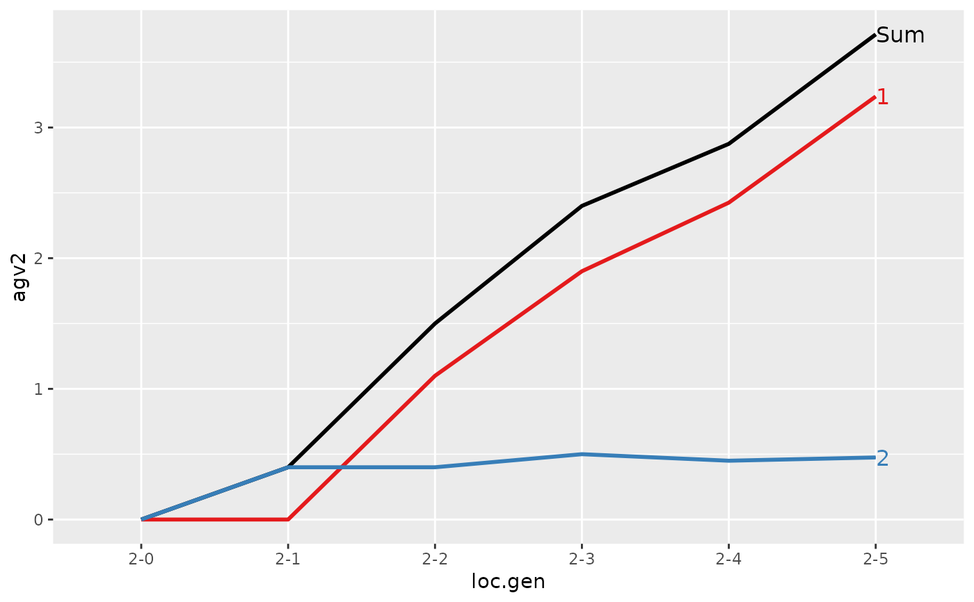
#> loc.gen N Sum 1 2
#> 1 1-0 2 2.0000 2.0000 0.000
#> 2 1-1 2 2.4000 2.4000 0.000
#> 3 1-2 2 2.8500 2.8500 0.000
#> 4 1-3 2 3.2500 3.2500 0.000
#> 5 1-4 2 4.0500 4.0500 0.000
#> 6 1-5 2 4.9500 4.9500 0.000
#> 7 2-0 2 0.0000 0.0000 0.000
#> 8 2-1 2 0.4000 0.0000 0.400
#> 9 2-2 2 1.5000 1.1000 0.400
#> 10 2-3 2 2.4000 1.9000 0.500
#> 11 2-4 2 2.8750 2.4250 0.450
#> 12 2-5 2 3.7125 3.2375 0.475
#>
#>
#> > plot(ret)
#>
#> > ## Summarize and plot location specific trends
#> > (ret <- summary(res, by="loc.gen"))
#>
#>
#> Summary of partitions of breeding values
#> - paths: 2 (1, 2)
#> - traits: 2 (agv1, agv2)
#>
#> Trait: agv1
#>
#> loc.gen N Sum 1 2
#> 1 1-0 2 2.000 2.0000 0.0000
#> 2 1-1 2 2.400 2.4000 0.0000
#> 3 1-2 2 2.850 2.8500 0.0000
#> 4 1-3 2 3.250 3.2500 0.0000
#> 5 1-4 2 4.050 4.0500 0.0000
#> 6 1-5 2 4.950 4.9500 0.0000
#> 7 2-0 2 0.000 0.0000 0.0000
#> 8 2-1 2 -0.200 0.0000 -0.2000
#> 9 2-2 2 1.000 1.1000 -0.1000
#> 10 2-3 2 1.850 1.9000 -0.0500
#> 11 2-4 2 2.500 2.4250 0.0750
#> 12 2-5 2 3.325 3.2375 0.0875
#>
#> Trait: agv2
#>
#> loc.gen N Sum 1 2
#> 1 1-0 2 2.0000 2.0000 0.000
#> 2 1-1 2 2.4000 2.4000 0.000
#> 3 1-2 2 2.8500 2.8500 0.000
#> 4 1-3 2 3.2500 3.2500 0.000
#> 5 1-4 2 4.0500 4.0500 0.000
#> 6 1-5 2 4.9500 4.9500 0.000
#> 7 2-0 2 0.0000 0.0000 0.000
#> 8 2-1 2 0.4000 0.0000 0.400
#> 9 2-2 2 1.5000 1.1000 0.400
#> 10 2-3 2 2.4000 1.9000 0.500
#> 11 2-4 2 2.8750 2.4250 0.450
#> 12 2-5 2 3.7125 3.2375 0.475
#>
#>
#> > plot(ret)
 #>
#> > ## Summarize and plot location specific trends but only for location 1
#> > (ret <- summary(res, by="loc.gen", subset=res[[1]]$loc == 1))
#>
#>
#> Summary of partitions of breeding values
#> - paths: 2 (1, 2)
#> - traits: 2 (agv1, agv2)
#>
#> Trait: agv1
#>
#> loc.gen N Sum 1 2
#> 1 1-0 2 2.00 2.00 0
#> 2 1-1 2 2.40 2.40 0
#> 3 1-2 2 2.85 2.85 0
#> 4 1-3 2 3.25 3.25 0
#> 5 1-4 2 4.05 4.05 0
#> 6 1-5 2 4.95 4.95 0
#>
#> Trait: agv2
#>
#> loc.gen N Sum 1 2
#> 1 1-0 2 2.00 2.00 0
#> 2 1-1 2 2.40 2.40 0
#> 3 1-2 2 2.85 2.85 0
#> 4 1-3 2 3.25 3.25 0
#> 5 1-4 2 4.05 4.05 0
#> 6 1-5 2 4.95 4.95 0
#>
#>
#> > plot(ret)
#>
#> > ## Summarize and plot location specific trends but only for location 1
#> > (ret <- summary(res, by="loc.gen", subset=res[[1]]$loc == 1))
#>
#>
#> Summary of partitions of breeding values
#> - paths: 2 (1, 2)
#> - traits: 2 (agv1, agv2)
#>
#> Trait: agv1
#>
#> loc.gen N Sum 1 2
#> 1 1-0 2 2.00 2.00 0
#> 2 1-1 2 2.40 2.40 0
#> 3 1-2 2 2.85 2.85 0
#> 4 1-3 2 3.25 3.25 0
#> 5 1-4 2 4.05 4.05 0
#> 6 1-5 2 4.95 4.95 0
#>
#> Trait: agv2
#>
#> loc.gen N Sum 1 2
#> 1 1-0 2 2.00 2.00 0
#> 2 1-1 2 2.40 2.40 0
#> 3 1-2 2 2.85 2.85 0
#> 4 1-3 2 3.25 3.25 0
#> 5 1-4 2 4.05 4.05 0
#> 6 1-5 2 4.95 4.95 0
#>
#>
#> > plot(ret)
 #>
#> > ## Summarize and plot location specific trends but only for location 2
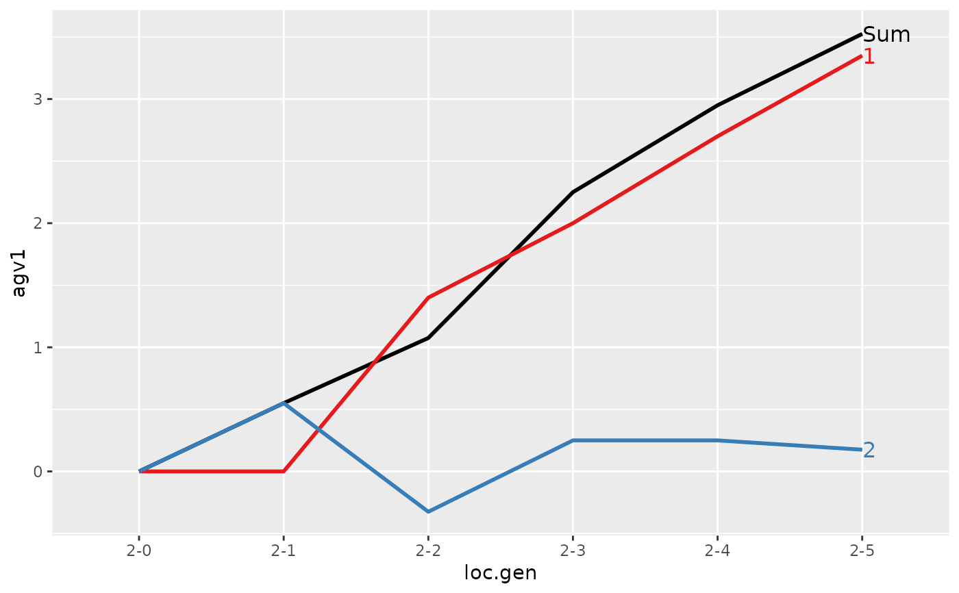
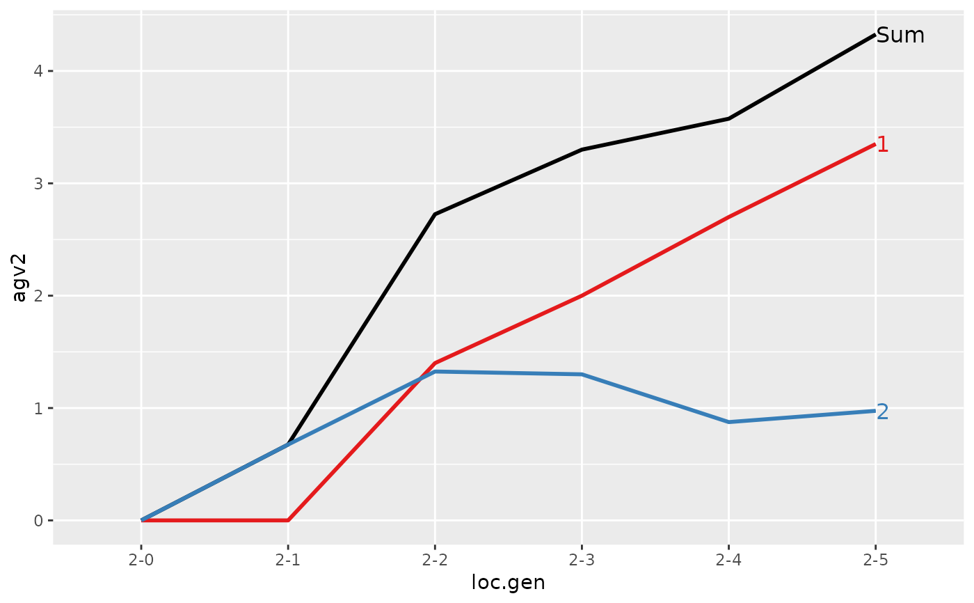
#> > (ret <- summary(res, by="loc.gen", subset=res[[1]]$loc == 2))
#>
#>
#> Summary of partitions of breeding values
#> - paths: 2 (1, 2)
#> - traits: 2 (agv1, agv2)
#>
#> Trait: agv1
#>
#> loc.gen N Sum 1 2
#> 1 2-0 2 0.000 0.0000 0.0000
#> 2 2-1 2 -0.200 0.0000 -0.2000
#> 3 2-2 2 1.000 1.1000 -0.1000
#> 4 2-3 2 1.850 1.9000 -0.0500
#> 5 2-4 2 2.500 2.4250 0.0750
#> 6 2-5 2 3.325 3.2375 0.0875
#>
#> Trait: agv2
#>
#> loc.gen N Sum 1 2
#> 1 2-0 2 0.0000 0.0000 0.000
#> 2 2-1 2 0.4000 0.0000 0.400
#> 3 2-2 2 1.5000 1.1000 0.400
#> 4 2-3 2 2.4000 1.9000 0.500
#> 5 2-4 2 2.8750 2.4250 0.450
#> 6 2-5 2 3.7125 3.2375 0.475
#>
#>
#> > plot(ret)
#>
#> > ## Summarize and plot location specific trends but only for location 2
#> > (ret <- summary(res, by="loc.gen", subset=res[[1]]$loc == 2))
#>
#>
#> Summary of partitions of breeding values
#> - paths: 2 (1, 2)
#> - traits: 2 (agv1, agv2)
#>
#> Trait: agv1
#>
#> loc.gen N Sum 1 2
#> 1 2-0 2 0.000 0.0000 0.0000
#> 2 2-1 2 -0.200 0.0000 -0.2000
#> 3 2-2 2 1.000 1.1000 -0.1000
#> 4 2-3 2 1.850 1.9000 -0.0500
#> 5 2-4 2 2.500 2.4250 0.0750
#> 6 2-5 2 3.325 3.2375 0.0875
#>
#> Trait: agv2
#>
#> loc.gen N Sum 1 2
#> 1 2-0 2 0.0000 0.0000 0.000
#> 2 2-1 2 0.4000 0.0000 0.400
#> 3 2-2 2 1.5000 1.1000 0.400
#> 4 2-3 2 2.4000 1.9000 0.500
#> 5 2-4 2 2.8750 2.4250 0.450
#> 6 2-5 2 3.7125 3.2375 0.475
#>
#>
#> > plot(ret)
 #>
#> > ## Compute partitions by location and sex
#> > ped$loc.sex <- with(ped, paste(loc, sex, sep="-"))
#>
#> > (res <- AlphaPart(x=ped, colPath="loc.sex", colBV=c("agv1", "agv2")))
#>
#> Size:
#> - individuals: 24
#> - traits: 2 (agv1, agv2)
#> - paths: 4 (1-1, 1-2, 2-1, 2-2)
#> - unknown (missing) values:
#> agv1 agv2
#> 0 0
#>
#>
#> Partitions of breeding values
#> - individuals: 24
#> - paths: 4 (1-1, 1-2, 2-1, 2-2)
#> - traits: 2 (agv1, agv2)
#>
#> Trait: agv1
#>
#> id fid mid loc gen w1 w2 sex loc.gen pa1 pa2 loc.sex agv1 agv1_pa agv1_w agv1_1-1 agv1_1-2 agv1_2-1 agv1_2-2
#> 1 01 <NA> <NA> 1 0 2.0 2.0 1 1-0 0 0 1-1 2.0 0 2.0 2.0 0.0 0 0
#> 2 02 <NA> <NA> 1 0 2.0 2.0 2 1-0 0 0 1-2 2.0 0 2.0 0.0 2.0 0 0
#> 3 03 <NA> <NA> 2 0 0.0 0.0 1 2-0 0 0 2-1 0.0 0 0.0 0.0 0.0 0 0
#> 4 04 <NA> <NA> 2 0 0.0 0.0 2 2-0 0 0 2-2 0.0 0 0.0 0.0 0.0 0 0
#> 5 11 01 02 1 1 0.6 0.6 2 1-1 2 2 1-2 2.6 2 0.6 1.0 1.6 0 0
#> 6 12 01 02 1 1 0.2 0.2 1 1-1 2 2 1-1 2.2 2 0.2 1.2 1.0 0 0
#> ...
#> id fid mid loc gen w1 w2 sex loc.gen pa1 pa2 loc.sex agv1 agv1_pa agv1_w agv1_1-1 agv1_1-2 agv1_2-1 agv1_2-2
#> 19 43 32 33 2 4 -0.1 0.1 2 2-4 2.15 2.700 2-2 2.05 2.15 -0.1 1.1750 1.25 0 -0.3750
#> 20 44 32 34 2 4 0.3 0.3 2 2-4 2.65 2.650 2-2 2.95 2.65 0.3 1.1750 1.25 0 0.5250
#> 21 51 42 41 1 5 0.8 0.8 2 1-5 4.05 4.050 1-2 4.85 4.05 0.8 1.7000 3.15 0 0.0000
#> 22 52 42 41 1 5 1.0 1.0 2 1-5 4.05 4.050 1-2 5.05 4.05 1.0 1.7000 3.35 0 0.0000
#> 23 53 42 43 2 5 -0.2 0.2 2 2-5 3.05 3.425 2-2 2.85 3.05 -0.2 1.6375 1.60 0 -0.3875
#> 24 54 42 44 2 5 0.3 0.3 2 2-5 3.50 3.500 2-2 3.80 3.50 0.3 1.6375 1.60 0 0.5625
#>
#> Trait: agv2
#>
#> id fid mid loc gen w1 w2 sex loc.gen pa1 pa2 loc.sex agv2 agv2_pa agv2_w agv2_1-1 agv2_1-2 agv2_2-1 agv2_2-2
#> 1 01 <NA> <NA> 1 0 2.0 2.0 1 1-0 0 0 1-1 2.0 0 2.0 2.0 0.0 0 0
#> 2 02 <NA> <NA> 1 0 2.0 2.0 2 1-0 0 0 1-2 2.0 0 2.0 0.0 2.0 0 0
#> 3 03 <NA> <NA> 2 0 0.0 0.0 1 2-0 0 0 2-1 0.0 0 0.0 0.0 0.0 0 0
#> 4 04 <NA> <NA> 2 0 0.0 0.0 2 2-0 0 0 2-2 0.0 0 0.0 0.0 0.0 0 0
#> 5 11 01 02 1 1 0.6 0.6 2 1-1 2 2 1-2 2.6 2 0.6 1.0 1.6 0 0
#> 6 12 01 02 1 1 0.2 0.2 1 1-1 2 2 1-1 2.2 2 0.2 1.2 1.0 0 0
#> ...
#> id fid mid loc gen w1 w2 sex loc.gen pa1 pa2 loc.sex agv2 agv2_pa agv2_w agv2_1-1 agv2_1-2 agv2_2-1 agv2_2-2
#> 19 43 32 33 2 4 -0.1 0.1 2 2-4 2.15 2.700 2-2 2.800 2.700 0.1 1.1750 1.25 0 0.3750
#> 20 44 32 34 2 4 0.3 0.3 2 2-4 2.65 2.650 2-2 2.950 2.650 0.3 1.1750 1.25 0 0.5250
#> 21 51 42 41 1 5 0.8 0.8 2 1-5 4.05 4.050 1-2 4.850 4.050 0.8 1.7000 3.15 0 0.0000
#> 22 52 42 41 1 5 1.0 1.0 2 1-5 4.05 4.050 1-2 5.050 4.050 1.0 1.7000 3.35 0 0.0000
#> 23 53 42 43 2 5 -0.2 0.2 2 2-5 3.05 3.425 2-2 3.625 3.425 0.2 1.6375 1.60 0 0.3875
#> 24 54 42 44 2 5 0.3 0.3 2 2-5 3.50 3.500 2-2 3.800 3.500 0.3 1.6375 1.60 0 0.5625
#>
#>
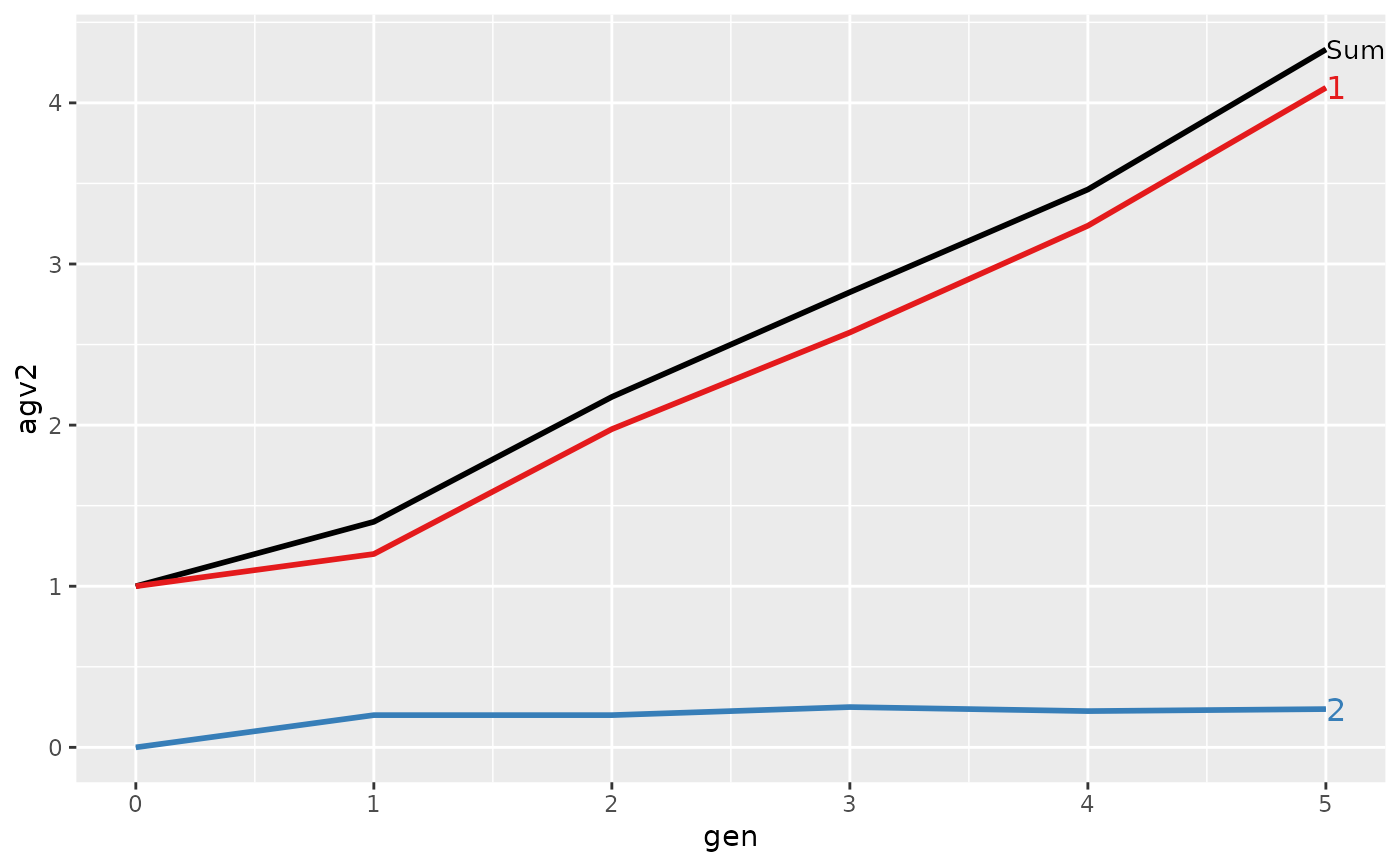
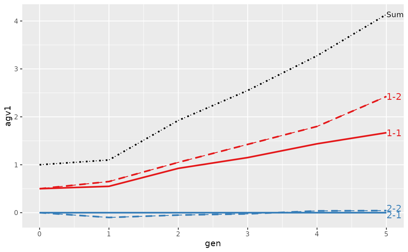
#> > ## Summarize and plot by generation (=trend)
#> > (ret <- summary(res, by="gen"))
#>
#>
#> Summary of partitions of breeding values
#> - paths: 4 (1-1, 1-2, 2-1, 2-2)
#> - traits: 2 (agv1, agv2)
#>
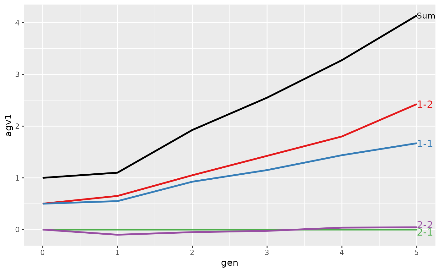
#> Trait: agv1
#>
#> gen N Sum 1-1 1-2 2-1 2-2
#> 1 0 4 1.0000 0.50000 0.500 0 0.00000
#> 2 1 4 1.1000 0.55000 0.650 0 -0.10000
#> 3 2 4 1.9250 0.92500 1.050 0 -0.05000
#> 4 3 4 2.5500 1.15000 1.425 0 -0.02500
#> 5 4 4 3.2750 1.43750 1.800 0 0.03750
#> 6 5 4 4.1375 1.66875 2.425 0 0.04375
#>
#> Trait: agv2
#>
#> gen N Sum 1-1 1-2 2-1 2-2
#> 1 0 4 1.00000 0.50000 0.500 0 0.0000
#> 2 1 4 1.40000 0.55000 0.650 0 0.2000
#> 3 2 4 2.17500 0.92500 1.050 0 0.2000
#> 4 3 4 2.82500 1.15000 1.425 0 0.2500
#> 5 4 4 3.46250 1.43750 1.800 0 0.2250
#> 6 5 4 4.33125 1.66875 2.425 0 0.2375
#>
#>
#> > plot(ret)
#>
#> > ## Compute partitions by location and sex
#> > ped$loc.sex <- with(ped, paste(loc, sex, sep="-"))
#>
#> > (res <- AlphaPart(x=ped, colPath="loc.sex", colBV=c("agv1", "agv2")))
#>
#> Size:
#> - individuals: 24
#> - traits: 2 (agv1, agv2)
#> - paths: 4 (1-1, 1-2, 2-1, 2-2)
#> - unknown (missing) values:
#> agv1 agv2
#> 0 0
#>
#>
#> Partitions of breeding values
#> - individuals: 24
#> - paths: 4 (1-1, 1-2, 2-1, 2-2)
#> - traits: 2 (agv1, agv2)
#>
#> Trait: agv1
#>
#> id fid mid loc gen w1 w2 sex loc.gen pa1 pa2 loc.sex agv1 agv1_pa agv1_w agv1_1-1 agv1_1-2 agv1_2-1 agv1_2-2
#> 1 01 <NA> <NA> 1 0 2.0 2.0 1 1-0 0 0 1-1 2.0 0 2.0 2.0 0.0 0 0
#> 2 02 <NA> <NA> 1 0 2.0 2.0 2 1-0 0 0 1-2 2.0 0 2.0 0.0 2.0 0 0
#> 3 03 <NA> <NA> 2 0 0.0 0.0 1 2-0 0 0 2-1 0.0 0 0.0 0.0 0.0 0 0
#> 4 04 <NA> <NA> 2 0 0.0 0.0 2 2-0 0 0 2-2 0.0 0 0.0 0.0 0.0 0 0
#> 5 11 01 02 1 1 0.6 0.6 2 1-1 2 2 1-2 2.6 2 0.6 1.0 1.6 0 0
#> 6 12 01 02 1 1 0.2 0.2 1 1-1 2 2 1-1 2.2 2 0.2 1.2 1.0 0 0
#> ...
#> id fid mid loc gen w1 w2 sex loc.gen pa1 pa2 loc.sex agv1 agv1_pa agv1_w agv1_1-1 agv1_1-2 agv1_2-1 agv1_2-2
#> 19 43 32 33 2 4 -0.1 0.1 2 2-4 2.15 2.700 2-2 2.05 2.15 -0.1 1.1750 1.25 0 -0.3750
#> 20 44 32 34 2 4 0.3 0.3 2 2-4 2.65 2.650 2-2 2.95 2.65 0.3 1.1750 1.25 0 0.5250
#> 21 51 42 41 1 5 0.8 0.8 2 1-5 4.05 4.050 1-2 4.85 4.05 0.8 1.7000 3.15 0 0.0000
#> 22 52 42 41 1 5 1.0 1.0 2 1-5 4.05 4.050 1-2 5.05 4.05 1.0 1.7000 3.35 0 0.0000
#> 23 53 42 43 2 5 -0.2 0.2 2 2-5 3.05 3.425 2-2 2.85 3.05 -0.2 1.6375 1.60 0 -0.3875
#> 24 54 42 44 2 5 0.3 0.3 2 2-5 3.50 3.500 2-2 3.80 3.50 0.3 1.6375 1.60 0 0.5625
#>
#> Trait: agv2
#>
#> id fid mid loc gen w1 w2 sex loc.gen pa1 pa2 loc.sex agv2 agv2_pa agv2_w agv2_1-1 agv2_1-2 agv2_2-1 agv2_2-2
#> 1 01 <NA> <NA> 1 0 2.0 2.0 1 1-0 0 0 1-1 2.0 0 2.0 2.0 0.0 0 0
#> 2 02 <NA> <NA> 1 0 2.0 2.0 2 1-0 0 0 1-2 2.0 0 2.0 0.0 2.0 0 0
#> 3 03 <NA> <NA> 2 0 0.0 0.0 1 2-0 0 0 2-1 0.0 0 0.0 0.0 0.0 0 0
#> 4 04 <NA> <NA> 2 0 0.0 0.0 2 2-0 0 0 2-2 0.0 0 0.0 0.0 0.0 0 0
#> 5 11 01 02 1 1 0.6 0.6 2 1-1 2 2 1-2 2.6 2 0.6 1.0 1.6 0 0
#> 6 12 01 02 1 1 0.2 0.2 1 1-1 2 2 1-1 2.2 2 0.2 1.2 1.0 0 0
#> ...
#> id fid mid loc gen w1 w2 sex loc.gen pa1 pa2 loc.sex agv2 agv2_pa agv2_w agv2_1-1 agv2_1-2 agv2_2-1 agv2_2-2
#> 19 43 32 33 2 4 -0.1 0.1 2 2-4 2.15 2.700 2-2 2.800 2.700 0.1 1.1750 1.25 0 0.3750
#> 20 44 32 34 2 4 0.3 0.3 2 2-4 2.65 2.650 2-2 2.950 2.650 0.3 1.1750 1.25 0 0.5250
#> 21 51 42 41 1 5 0.8 0.8 2 1-5 4.05 4.050 1-2 4.850 4.050 0.8 1.7000 3.15 0 0.0000
#> 22 52 42 41 1 5 1.0 1.0 2 1-5 4.05 4.050 1-2 5.050 4.050 1.0 1.7000 3.35 0 0.0000
#> 23 53 42 43 2 5 -0.2 0.2 2 2-5 3.05 3.425 2-2 3.625 3.425 0.2 1.6375 1.60 0 0.3875
#> 24 54 42 44 2 5 0.3 0.3 2 2-5 3.50 3.500 2-2 3.800 3.500 0.3 1.6375 1.60 0 0.5625
#>
#>
#> > ## Summarize and plot by generation (=trend)
#> > (ret <- summary(res, by="gen"))
#>
#>
#> Summary of partitions of breeding values
#> - paths: 4 (1-1, 1-2, 2-1, 2-2)
#> - traits: 2 (agv1, agv2)
#>
#> Trait: agv1
#>
#> gen N Sum 1-1 1-2 2-1 2-2
#> 1 0 4 1.0000 0.50000 0.500 0 0.00000
#> 2 1 4 1.1000 0.55000 0.650 0 -0.10000
#> 3 2 4 1.9250 0.92500 1.050 0 -0.05000
#> 4 3 4 2.5500 1.15000 1.425 0 -0.02500
#> 5 4 4 3.2750 1.43750 1.800 0 0.03750
#> 6 5 4 4.1375 1.66875 2.425 0 0.04375
#>
#> Trait: agv2
#>
#> gen N Sum 1-1 1-2 2-1 2-2
#> 1 0 4 1.00000 0.50000 0.500 0 0.0000
#> 2 1 4 1.40000 0.55000 0.650 0 0.2000
#> 3 2 4 2.17500 0.92500 1.050 0 0.2000
#> 4 3 4 2.82500 1.15000 1.425 0 0.2500
#> 5 4 4 3.46250 1.43750 1.800 0 0.2250
#> 6 5 4 4.33125 1.66875 2.425 0 0.2375
#>
#>
#> > plot(ret)
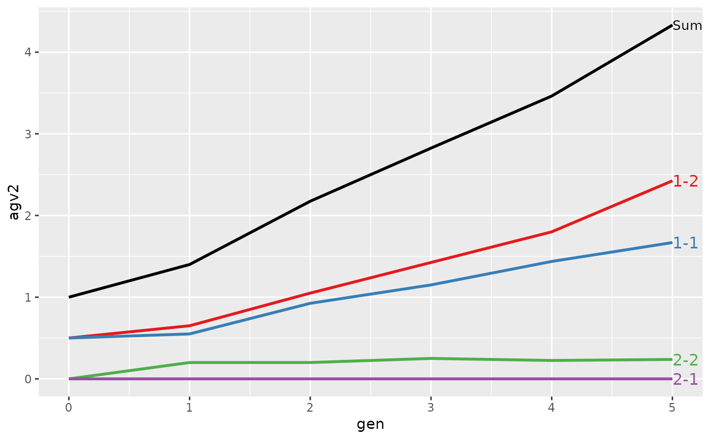 #>
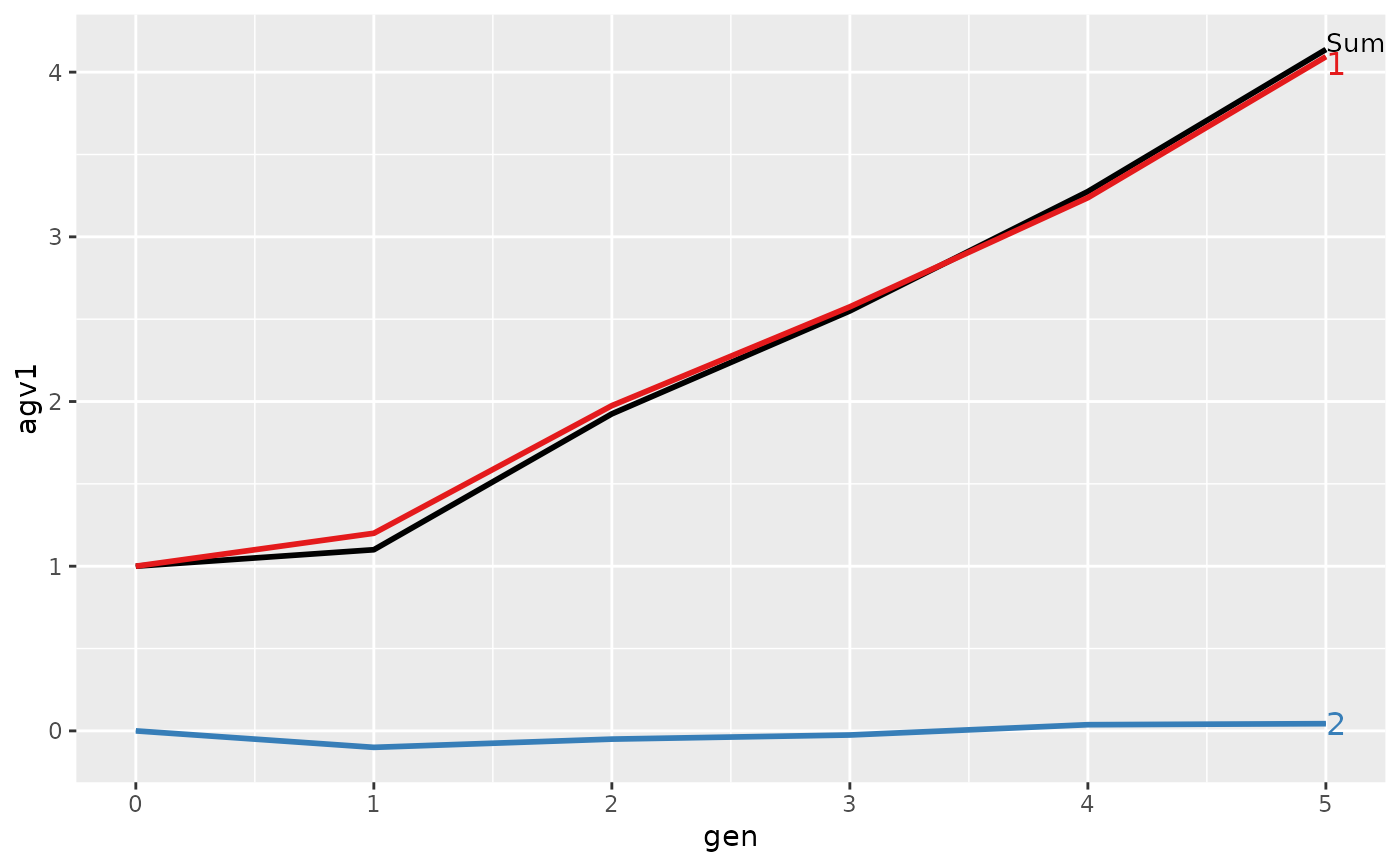
#> > plot(ret, lineTypeList=list("-1"=1, "-2"=2, def=3))
#>
#> > plot(ret, lineTypeList=list("-1"=1, "-2"=2, def=3))
 #>
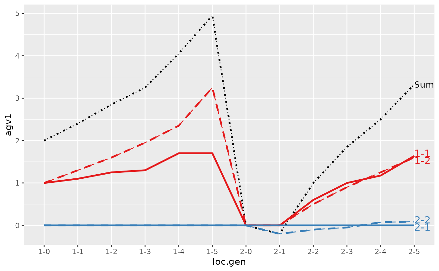
#> > ## Summarize and plot location specific trends
#> > (ret <- summary(res, by="loc.gen"))
#>
#>
#> Summary of partitions of breeding values
#> - paths: 4 (1-1, 1-2, 2-1, 2-2)
#> - traits: 2 (agv1, agv2)
#>
#> Trait: agv1
#>
#> loc.gen N Sum 1-1 1-2 2-1 2-2
#> 1 1-0 2 2.000 1.0000 1.00 0 0.0000
#> 2 1-1 2 2.400 1.1000 1.30 0 0.0000
#> 3 1-2 2 2.850 1.2500 1.60 0 0.0000
#> 4 1-3 2 3.250 1.3000 1.95 0 0.0000
#> 5 1-4 2 4.050 1.7000 2.35 0 0.0000
#> 6 1-5 2 4.950 1.7000 3.25 0 0.0000
#> 7 2-0 2 0.000 0.0000 0.00 0 0.0000
#> 8 2-1 2 -0.200 0.0000 0.00 0 -0.2000
#> 9 2-2 2 1.000 0.6000 0.50 0 -0.1000
#> 10 2-3 2 1.850 1.0000 0.90 0 -0.0500
#> 11 2-4 2 2.500 1.1750 1.25 0 0.0750
#> 12 2-5 2 3.325 1.6375 1.60 0 0.0875
#>
#> Trait: agv2
#>
#> loc.gen N Sum 1-1 1-2 2-1 2-2
#> 1 1-0 2 2.0000 1.0000 1.00 0 0.000
#> 2 1-1 2 2.4000 1.1000 1.30 0 0.000
#> 3 1-2 2 2.8500 1.2500 1.60 0 0.000
#> 4 1-3 2 3.2500 1.3000 1.95 0 0.000
#> 5 1-4 2 4.0500 1.7000 2.35 0 0.000
#> 6 1-5 2 4.9500 1.7000 3.25 0 0.000
#> 7 2-0 2 0.0000 0.0000 0.00 0 0.000
#> 8 2-1 2 0.4000 0.0000 0.00 0 0.400
#> 9 2-2 2 1.5000 0.6000 0.50 0 0.400
#> 10 2-3 2 2.4000 1.0000 0.90 0 0.500
#> 11 2-4 2 2.8750 1.1750 1.25 0 0.450
#> 12 2-5 2 3.7125 1.6375 1.60 0 0.475
#>
#>
#> > plot(ret, lineTypeList=list("-1"=1, "-2"=2, def=3))
#>
#> > ## Summarize and plot location specific trends
#> > (ret <- summary(res, by="loc.gen"))
#>
#>
#> Summary of partitions of breeding values
#> - paths: 4 (1-1, 1-2, 2-1, 2-2)
#> - traits: 2 (agv1, agv2)
#>
#> Trait: agv1
#>
#> loc.gen N Sum 1-1 1-2 2-1 2-2
#> 1 1-0 2 2.000 1.0000 1.00 0 0.0000
#> 2 1-1 2 2.400 1.1000 1.30 0 0.0000
#> 3 1-2 2 2.850 1.2500 1.60 0 0.0000
#> 4 1-3 2 3.250 1.3000 1.95 0 0.0000
#> 5 1-4 2 4.050 1.7000 2.35 0 0.0000
#> 6 1-5 2 4.950 1.7000 3.25 0 0.0000
#> 7 2-0 2 0.000 0.0000 0.00 0 0.0000
#> 8 2-1 2 -0.200 0.0000 0.00 0 -0.2000
#> 9 2-2 2 1.000 0.6000 0.50 0 -0.1000
#> 10 2-3 2 1.850 1.0000 0.90 0 -0.0500
#> 11 2-4 2 2.500 1.1750 1.25 0 0.0750
#> 12 2-5 2 3.325 1.6375 1.60 0 0.0875
#>
#> Trait: agv2
#>
#> loc.gen N Sum 1-1 1-2 2-1 2-2
#> 1 1-0 2 2.0000 1.0000 1.00 0 0.000
#> 2 1-1 2 2.4000 1.1000 1.30 0 0.000
#> 3 1-2 2 2.8500 1.2500 1.60 0 0.000
#> 4 1-3 2 3.2500 1.3000 1.95 0 0.000
#> 5 1-4 2 4.0500 1.7000 2.35 0 0.000
#> 6 1-5 2 4.9500 1.7000 3.25 0 0.000
#> 7 2-0 2 0.0000 0.0000 0.00 0 0.000
#> 8 2-1 2 0.4000 0.0000 0.00 0 0.400
#> 9 2-2 2 1.5000 0.6000 0.50 0 0.400
#> 10 2-3 2 2.4000 1.0000 0.90 0 0.500
#> 11 2-4 2 2.8750 1.1750 1.25 0 0.450
#> 12 2-5 2 3.7125 1.6375 1.60 0 0.475
#>
#>
#> > plot(ret, lineTypeList=list("-1"=1, "-2"=2, def=3))
 #>
#> > ## Summarize and plot location specific trends but only for location 1
#> > (ret <- summary(res, by="loc.gen", subset=res[[1]]$loc == 1))
#>
#>
#> Summary of partitions of breeding values
#> - paths: 4 (1-1, 1-2, 2-1, 2-2)
#> - traits: 2 (agv1, agv2)
#>
#> Trait: agv1
#>
#> loc.gen N Sum 1-1 1-2 2-1 2-2
#> 1 1-0 2 2.00 1.00 1.00 0 0
#> 2 1-1 2 2.40 1.10 1.30 0 0
#> 3 1-2 2 2.85 1.25 1.60 0 0
#> 4 1-3 2 3.25 1.30 1.95 0 0
#> 5 1-4 2 4.05 1.70 2.35 0 0
#> 6 1-5 2 4.95 1.70 3.25 0 0
#>
#> Trait: agv2
#>
#> loc.gen N Sum 1-1 1-2 2-1 2-2
#> 1 1-0 2 2.00 1.00 1.00 0 0
#> 2 1-1 2 2.40 1.10 1.30 0 0
#> 3 1-2 2 2.85 1.25 1.60 0 0
#> 4 1-3 2 3.25 1.30 1.95 0 0
#> 5 1-4 2 4.05 1.70 2.35 0 0
#> 6 1-5 2 4.95 1.70 3.25 0 0
#>
#>
#> > plot(ret)
#>
#> > ## Summarize and plot location specific trends but only for location 1
#> > (ret <- summary(res, by="loc.gen", subset=res[[1]]$loc == 1))
#>
#>
#> Summary of partitions of breeding values
#> - paths: 4 (1-1, 1-2, 2-1, 2-2)
#> - traits: 2 (agv1, agv2)
#>
#> Trait: agv1
#>
#> loc.gen N Sum 1-1 1-2 2-1 2-2
#> 1 1-0 2 2.00 1.00 1.00 0 0
#> 2 1-1 2 2.40 1.10 1.30 0 0
#> 3 1-2 2 2.85 1.25 1.60 0 0
#> 4 1-3 2 3.25 1.30 1.95 0 0
#> 5 1-4 2 4.05 1.70 2.35 0 0
#> 6 1-5 2 4.95 1.70 3.25 0 0
#>
#> Trait: agv2
#>
#> loc.gen N Sum 1-1 1-2 2-1 2-2
#> 1 1-0 2 2.00 1.00 1.00 0 0
#> 2 1-1 2 2.40 1.10 1.30 0 0
#> 3 1-2 2 2.85 1.25 1.60 0 0
#> 4 1-3 2 3.25 1.30 1.95 0 0
#> 5 1-4 2 4.05 1.70 2.35 0 0
#> 6 1-5 2 4.95 1.70 3.25 0 0
#>
#>
#> > plot(ret)
 #>
#> > ## Summarize and plot location specific trends but only for location 2
#> > (ret <- summary(res, by="loc.gen", subset=res[[1]]$loc == 2))
#>
#>
#> Summary of partitions of breeding values
#> - paths: 4 (1-1, 1-2, 2-1, 2-2)
#> - traits: 2 (agv1, agv2)
#>
#> Trait: agv1
#>
#> loc.gen N Sum 1-1 1-2 2-1 2-2
#> 1 2-0 2 0.000 0.0000 0.00 0 0.0000
#> 2 2-1 2 -0.200 0.0000 0.00 0 -0.2000
#> 3 2-2 2 1.000 0.6000 0.50 0 -0.1000
#> 4 2-3 2 1.850 1.0000 0.90 0 -0.0500
#> 5 2-4 2 2.500 1.1750 1.25 0 0.0750
#> 6 2-5 2 3.325 1.6375 1.60 0 0.0875
#>
#> Trait: agv2
#>
#> loc.gen N Sum 1-1 1-2 2-1 2-2
#> 1 2-0 2 0.0000 0.0000 0.00 0 0.000
#> 2 2-1 2 0.4000 0.0000 0.00 0 0.400
#> 3 2-2 2 1.5000 0.6000 0.50 0 0.400
#> 4 2-3 2 2.4000 1.0000 0.90 0 0.500
#> 5 2-4 2 2.8750 1.1750 1.25 0 0.450
#> 6 2-5 2 3.7125 1.6375 1.60 0 0.475
#>
#>
#> > plot(ret)
#>
#> > ## Summarize and plot location specific trends but only for location 2
#> > (ret <- summary(res, by="loc.gen", subset=res[[1]]$loc == 2))
#>
#>
#> Summary of partitions of breeding values
#> - paths: 4 (1-1, 1-2, 2-1, 2-2)
#> - traits: 2 (agv1, agv2)
#>
#> Trait: agv1
#>
#> loc.gen N Sum 1-1 1-2 2-1 2-2
#> 1 2-0 2 0.000 0.0000 0.00 0 0.0000
#> 2 2-1 2 -0.200 0.0000 0.00 0 -0.2000
#> 3 2-2 2 1.000 0.6000 0.50 0 -0.1000
#> 4 2-3 2 1.850 1.0000 0.90 0 -0.0500
#> 5 2-4 2 2.500 1.1750 1.25 0 0.0750
#> 6 2-5 2 3.325 1.6375 1.60 0 0.0875
#>
#> Trait: agv2
#>
#> loc.gen N Sum 1-1 1-2 2-1 2-2
#> 1 2-0 2 0.0000 0.0000 0.00 0 0.000
#> 2 2-1 2 0.4000 0.0000 0.00 0 0.400
#> 3 2-2 2 1.5000 0.6000 0.50 0 0.400
#> 4 2-3 2 2.4000 1.0000 0.90 0 0.500
#> 5 2-4 2 2.8750 1.1750 1.25 0 0.450
#> 6 2-5 2 3.7125 1.6375 1.60 0 0.475
#>
#>
#> > plot(ret)
 #>
#> > ###-----------------------------------------------------------------------------
#> > ### AlphaPart_deterministic.R ends here
demo(topic="AlphaPart_stochastic", package="AlphaPart",
ask=interactive())
#>
#>
#> demo(AlphaPart_stochastic)
#> ---- ~~~~~~~~~~~~~~~~~~~~
#>
#> > ### demo_stohastic.R
#> > ###-----------------------------------------------------------------------------
#> > ### $Id$
#> > ###-----------------------------------------------------------------------------
#> >
#> > ### DESCRIPTION OF A DEMONSTRATION
#> > ###-----------------------------------------------------------------------------
#> >
#> > ## A demonstration with a simple example to see in action the partitioning of
#> > ## additive genetic values by paths (Garcia-Cortes et al., 2008; Animal)
#> > ##
#> > ## STOHASTIC SIMULATION (sort of)
#> > ##
#> > ## We have two locations (1 and 2). The first location has individualss with higher
#> > ## additive genetic value. Males from the first location are imported males to the
#> > ## second location from generation 2/3. This clearly leads to genetic gain in the
#> > ## second location. However, the second location can also perform their own selection
#> > ## so the question is how much genetic gain is due to the import of genes from the
#> > ## first location and due to their own selection.
#> > ##
#> > ## Above scenario will be tested with a simple example of a pedigree bellow. Two
#> > ## scenarios will be evaluated: without or with own selection in the second location.
#> > ## Selection will always be present in the first location.
#> > ##
#> > ## Additive genetic values are provided, i.e., no inference is being done!
#> > ##
#> > ## The idea of this example is not to do extensive simulations, but just to have
#> > ## a simple example to see how the partitioning of additive genetic values works.
#> >
#> > ### SETUP
#> > ###-----------------------------------------------------------------------------
#> >
#> > options(width=200)
#>
#> > ## install.packages(pkg=c("truncnorm"), dep=TRUE)
#> > library(package="truncnorm")
#>
#> > ### EXAMPLE PEDIGREE
#> > ###-----------------------------------------------------------------------------
#> >
#> > ## Generation 0
#> > id0 <- c("01", "02", "03", "04", "05", "06", "07", "08")
#>
#> > fid0 <- mid0 <- rep(NA, times=length(id0))
#>
#> > h0 <- rep(c(1, 2), each=4)
#>
#> > g0 <- rep(0, times=length(id0))
#>
#> > ## Generation 1
#> > id1 <- c("11", "12", "13", "14", "15", "16", "17", "18")
#>
#> > fid1 <- c("02", "02", "02", "02", "06", "06", "06", "06")
#>
#> > mid1 <- c("01", "01", "03", "04", "05", "05", "07", "08")
#>
#> > h1 <- h0
#>
#> > g1 <- rep(1, times=length(id1))
#>
#> > ## Generation 2
#> > id2 <- c("21", "22", "23", "24", "25", "26", "27", "28")
#>
#> > fid2 <- c("13", "13", "13", "13", "13", "13", "13", "13")
#>
#> > mid2 <- c("11", "12", "14", "14", "15", "16", "17", "18")
#>
#> > h2 <- h0
#>
#> > g2 <- rep(2, times=length(id2))
#>
#> > ## Generation 3
#> > id3 <- c("31", "32", "33", "34", "35", "36", "37", "38")
#>
#> > fid3 <- c("24", "24", "24", "24", "24", "24", "24", "24")
#>
#> > mid3 <- c("21", "21", "22", "23", "25", "26", "27", "28")
#>
#> > h3 <- h0
#>
#> > g3 <- rep(3, times=length(id3))
#>
#> > ## Generation 4
#> > id4 <- c("41", "42", "43", "44", "45", "46", "47", "48")
#>
#> > fid4 <- c("34", "34", "34", "34", "34", "34", "34", "34")
#>
#> > mid4 <- c("31", "32", "32", "33", "35", "36", "37", "38")
#>
#> > h4 <- h0
#>
#> > g4 <- rep(4, times=length(id4))
#>
#> > ## Generation 5
#> > id5 <- c("51", "52", "53", "54", "55", "56", "57", "58")
#>
#> > fid5 <- c("44", "44", "44", "44", "44", "44", "44", "44")
#>
#> > mid5 <- c("41", "42", "43", "43", "45", "46", "47", "48")
#>
#> > h5 <- h0
#>
#> > g5 <- rep(5, times=length(id4))
#>
#> > ped <- data.frame( id=c( id0, id1, id2, id3, id4, id5),
#> + fid=c(fid0, fid1, fid2, fid3, fid4, fid5),
#> + mid=c(mid0, mid1, mid2, mid3, mid4, mid5),
#> + loc=c( h0, h1, h2, h3, h4, h5),
#> + gen=c( g0, g1, g2, g3, g4, g5))
#>
#> > ped$sex <- 2
#>
#> > ped[ped$id %in% ped$fid, "sex"] <- 1
#>
#> > ped$loc.gen <- with(ped, paste(loc, gen, sep="-"))
#>
#> > ### SIMULATE ADDITIVE GENETIC VALUES - STOHASTIC
#> > ###-----------------------------------------------------------------------------
#> >
#> > ## --- Parameters of simulation ---
#> >
#> > ## Additive genetic mean in founders by location
#> > mu1 <- 2
#>
#> > mu2 <- 0
#>
#> > ## Additive genetic variance in population
#> > sigma2 <- 1
#>
#> > sigma <- sqrt(sigma2)
#>
#> > ## Threshold value for Mendelian sampling for selection - only values above this
#> > ## will be accepted in simulation
#> > t <- 0
#>
#> > ## Set seed for simulation
#> > set.seed(seed=19791123)
#>
#> > ## --- Start of simulation ---
#> >
#> > ped$agv1 <- NA ## Scenario (trait) 1: No selection in the second location
#>
#> > ped$agv2 <- NA ## Scenario (trait) 2: Selection in the second location
#>
#> > ## Generation 0 - founders (for simplicity set their values to the mean of location)
#> > ped[ped$gen == 0 & ped$loc == 1, c("agv1", "agv2")] <- mu1
#>
#> > ped[ped$gen == 0 & ped$loc == 2, c("agv1", "agv2")] <- mu2
#>
#> > ## Generation 1+ - non-founders
#> > for(i in (length(g0)+1):nrow(ped)) {
#> + ## Scenario (trait) 1: selection only in the first location
#> + if(ped[i, "loc"] == 1) {
#> + w <- rtruncnorm(n=1, mean=0, sd=sqrt(sigma2/2), a=t)
#> + } else {
#> + w <- rnorm(n=1, mean=0, sd=sqrt(sigma2/2))
#> + }
#> + ped[i, "agv1"] <- round(0.5 * ped[ped$id %in% ped[i, "fid"], "agv1"] +
#> + 0.5 * ped[ped$id %in% ped[i, "mid"], "agv1"] +
#> + w, digits=1)
#> + ## Scenario (trait) 2: selection in both locations
#> + if(ped[i, "loc"] == 2) {
#> + w <- rtruncnorm(n=1, mean=0, sd=sqrt(sigma2/2), a=t)
#> + } ## for location 1 take the same values as above
#> + ped[i, "agv2"] <- round(0.5 * ped[ped$id %in% ped[i, "fid"], "agv2"] +
#> + 0.5 * ped[ped$id %in% ped[i, "mid"], "agv2"] +
#> + w, digits=1)
#> + }
#>
#> > ### PLOT INDIVIDUAL ADDITIVE GENETIC VALUES
#> > ###-----------------------------------------------------------------------------
#> >
#> > par(mfrow=c(2, 1), bty="l", pty="m", mar=c(2, 2, 1, 1) + .1, mgp=c(0.7, 0.2, 0))
#>
#> > tmp <- ped$gen + c(-1.5, -0.5, 0.5, 1.5) * 0.1
#>
#> > with(ped, plot(agv1 ~ tmp, pch=c(19, 21)[ped$loc], ylab="Additive genetic value",
#> + xlab="Generation", main="Selection in location 1", axes=FALSE,
#> + ylim=range(c(agv1, agv2))))
#>
#> > axis(1, labels=FALSE, tick=FALSE); axis(2, labels=FALSE, tick=FALSE); box()
#>
#> > legend(x="topleft", legend=c(1, 2), title="Location", pch=c(19, 21), bty="n")
#>
#> > with(ped, plot(agv2 ~ tmp, pch=c(19, 21)[ped$loc], ylab="Additive genetic value",
#> + xlab="Generation", main="Selection in locations 1 and 2", axes=FALSE,
#> + ylim=range(c(agv1, agv2))))
#>
#> > ###-----------------------------------------------------------------------------
#> > ### AlphaPart_deterministic.R ends here
demo(topic="AlphaPart_stochastic", package="AlphaPart",
ask=interactive())
#>
#>
#> demo(AlphaPart_stochastic)
#> ---- ~~~~~~~~~~~~~~~~~~~~
#>
#> > ### demo_stohastic.R
#> > ###-----------------------------------------------------------------------------
#> > ### $Id$
#> > ###-----------------------------------------------------------------------------
#> >
#> > ### DESCRIPTION OF A DEMONSTRATION
#> > ###-----------------------------------------------------------------------------
#> >
#> > ## A demonstration with a simple example to see in action the partitioning of
#> > ## additive genetic values by paths (Garcia-Cortes et al., 2008; Animal)
#> > ##
#> > ## STOHASTIC SIMULATION (sort of)
#> > ##
#> > ## We have two locations (1 and 2). The first location has individualss with higher
#> > ## additive genetic value. Males from the first location are imported males to the
#> > ## second location from generation 2/3. This clearly leads to genetic gain in the
#> > ## second location. However, the second location can also perform their own selection
#> > ## so the question is how much genetic gain is due to the import of genes from the
#> > ## first location and due to their own selection.
#> > ##
#> > ## Above scenario will be tested with a simple example of a pedigree bellow. Two
#> > ## scenarios will be evaluated: without or with own selection in the second location.
#> > ## Selection will always be present in the first location.
#> > ##
#> > ## Additive genetic values are provided, i.e., no inference is being done!
#> > ##
#> > ## The idea of this example is not to do extensive simulations, but just to have
#> > ## a simple example to see how the partitioning of additive genetic values works.
#> >
#> > ### SETUP
#> > ###-----------------------------------------------------------------------------
#> >
#> > options(width=200)
#>
#> > ## install.packages(pkg=c("truncnorm"), dep=TRUE)
#> > library(package="truncnorm")
#>
#> > ### EXAMPLE PEDIGREE
#> > ###-----------------------------------------------------------------------------
#> >
#> > ## Generation 0
#> > id0 <- c("01", "02", "03", "04", "05", "06", "07", "08")
#>
#> > fid0 <- mid0 <- rep(NA, times=length(id0))
#>
#> > h0 <- rep(c(1, 2), each=4)
#>
#> > g0 <- rep(0, times=length(id0))
#>
#> > ## Generation 1
#> > id1 <- c("11", "12", "13", "14", "15", "16", "17", "18")
#>
#> > fid1 <- c("02", "02", "02", "02", "06", "06", "06", "06")
#>
#> > mid1 <- c("01", "01", "03", "04", "05", "05", "07", "08")
#>
#> > h1 <- h0
#>
#> > g1 <- rep(1, times=length(id1))
#>
#> > ## Generation 2
#> > id2 <- c("21", "22", "23", "24", "25", "26", "27", "28")
#>
#> > fid2 <- c("13", "13", "13", "13", "13", "13", "13", "13")
#>
#> > mid2 <- c("11", "12", "14", "14", "15", "16", "17", "18")
#>
#> > h2 <- h0
#>
#> > g2 <- rep(2, times=length(id2))
#>
#> > ## Generation 3
#> > id3 <- c("31", "32", "33", "34", "35", "36", "37", "38")
#>
#> > fid3 <- c("24", "24", "24", "24", "24", "24", "24", "24")
#>
#> > mid3 <- c("21", "21", "22", "23", "25", "26", "27", "28")
#>
#> > h3 <- h0
#>
#> > g3 <- rep(3, times=length(id3))
#>
#> > ## Generation 4
#> > id4 <- c("41", "42", "43", "44", "45", "46", "47", "48")
#>
#> > fid4 <- c("34", "34", "34", "34", "34", "34", "34", "34")
#>
#> > mid4 <- c("31", "32", "32", "33", "35", "36", "37", "38")
#>
#> > h4 <- h0
#>
#> > g4 <- rep(4, times=length(id4))
#>
#> > ## Generation 5
#> > id5 <- c("51", "52", "53", "54", "55", "56", "57", "58")
#>
#> > fid5 <- c("44", "44", "44", "44", "44", "44", "44", "44")
#>
#> > mid5 <- c("41", "42", "43", "43", "45", "46", "47", "48")
#>
#> > h5 <- h0
#>
#> > g5 <- rep(5, times=length(id4))
#>
#> > ped <- data.frame( id=c( id0, id1, id2, id3, id4, id5),
#> + fid=c(fid0, fid1, fid2, fid3, fid4, fid5),
#> + mid=c(mid0, mid1, mid2, mid3, mid4, mid5),
#> + loc=c( h0, h1, h2, h3, h4, h5),
#> + gen=c( g0, g1, g2, g3, g4, g5))
#>
#> > ped$sex <- 2
#>
#> > ped[ped$id %in% ped$fid, "sex"] <- 1
#>
#> > ped$loc.gen <- with(ped, paste(loc, gen, sep="-"))
#>
#> > ### SIMULATE ADDITIVE GENETIC VALUES - STOHASTIC
#> > ###-----------------------------------------------------------------------------
#> >
#> > ## --- Parameters of simulation ---
#> >
#> > ## Additive genetic mean in founders by location
#> > mu1 <- 2
#>
#> > mu2 <- 0
#>
#> > ## Additive genetic variance in population
#> > sigma2 <- 1
#>
#> > sigma <- sqrt(sigma2)
#>
#> > ## Threshold value for Mendelian sampling for selection - only values above this
#> > ## will be accepted in simulation
#> > t <- 0
#>
#> > ## Set seed for simulation
#> > set.seed(seed=19791123)
#>
#> > ## --- Start of simulation ---
#> >
#> > ped$agv1 <- NA ## Scenario (trait) 1: No selection in the second location
#>
#> > ped$agv2 <- NA ## Scenario (trait) 2: Selection in the second location
#>
#> > ## Generation 0 - founders (for simplicity set their values to the mean of location)
#> > ped[ped$gen == 0 & ped$loc == 1, c("agv1", "agv2")] <- mu1
#>
#> > ped[ped$gen == 0 & ped$loc == 2, c("agv1", "agv2")] <- mu2
#>
#> > ## Generation 1+ - non-founders
#> > for(i in (length(g0)+1):nrow(ped)) {
#> + ## Scenario (trait) 1: selection only in the first location
#> + if(ped[i, "loc"] == 1) {
#> + w <- rtruncnorm(n=1, mean=0, sd=sqrt(sigma2/2), a=t)
#> + } else {
#> + w <- rnorm(n=1, mean=0, sd=sqrt(sigma2/2))
#> + }
#> + ped[i, "agv1"] <- round(0.5 * ped[ped$id %in% ped[i, "fid"], "agv1"] +
#> + 0.5 * ped[ped$id %in% ped[i, "mid"], "agv1"] +
#> + w, digits=1)
#> + ## Scenario (trait) 2: selection in both locations
#> + if(ped[i, "loc"] == 2) {
#> + w <- rtruncnorm(n=1, mean=0, sd=sqrt(sigma2/2), a=t)
#> + } ## for location 1 take the same values as above
#> + ped[i, "agv2"] <- round(0.5 * ped[ped$id %in% ped[i, "fid"], "agv2"] +
#> + 0.5 * ped[ped$id %in% ped[i, "mid"], "agv2"] +
#> + w, digits=1)
#> + }
#>
#> > ### PLOT INDIVIDUAL ADDITIVE GENETIC VALUES
#> > ###-----------------------------------------------------------------------------
#> >
#> > par(mfrow=c(2, 1), bty="l", pty="m", mar=c(2, 2, 1, 1) + .1, mgp=c(0.7, 0.2, 0))
#>
#> > tmp <- ped$gen + c(-1.5, -0.5, 0.5, 1.5) * 0.1
#>
#> > with(ped, plot(agv1 ~ tmp, pch=c(19, 21)[ped$loc], ylab="Additive genetic value",
#> + xlab="Generation", main="Selection in location 1", axes=FALSE,
#> + ylim=range(c(agv1, agv2))))
#>
#> > axis(1, labels=FALSE, tick=FALSE); axis(2, labels=FALSE, tick=FALSE); box()
#>
#> > legend(x="topleft", legend=c(1, 2), title="Location", pch=c(19, 21), bty="n")
#>
#> > with(ped, plot(agv2 ~ tmp, pch=c(19, 21)[ped$loc], ylab="Additive genetic value",
#> + xlab="Generation", main="Selection in locations 1 and 2", axes=FALSE,
#> + ylim=range(c(agv1, agv2))))
 #>
#> > axis(1, labels=FALSE, tick=FALSE); axis(2, labels=FALSE, tick=FALSE); box()
#>
#> > legend(x="topleft", legend=c(1, 2), title="Location", pch=c(19, 21), bty="n")
#>
#> > ### PARTITION ADDITIVE GENETIC VALUES BY ...
#> > ###-----------------------------------------------------------------------------
#> >
#> > ## Compute partitions by location
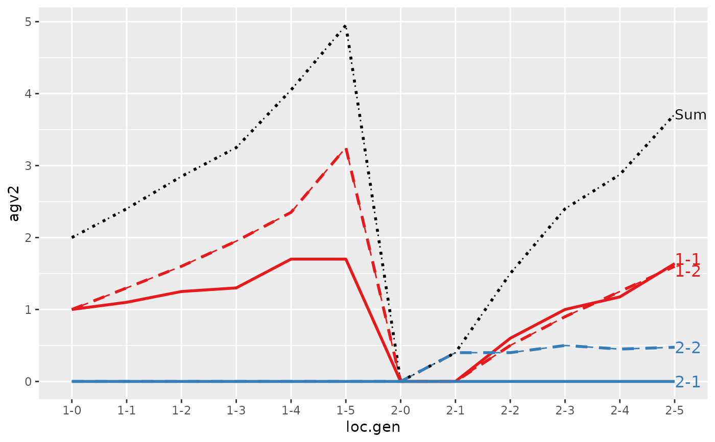
#> > (res <- AlphaPart(x=ped, colPath="loc", colBV=c("agv1", "agv2")))
#>
#> Size:
#> - individuals: 48
#> - traits: 2 (agv1, agv2)
#> - paths: 2 (1, 2)
#> - unknown (missing) values:
#> agv1 agv2
#> 0 0
#>
#>
#> Partitions of breeding values
#> - individuals: 48
#> - paths: 2 (1, 2)
#> - traits: 2 (agv1, agv2)
#>
#> Trait: agv1
#>
#> id fid mid loc gen sex loc.gen agv1 agv1_pa agv1_w agv1_1 agv1_2
#> 1 01 <NA> <NA> 1 0 2 1-0 2 1 1 2 0
#> 2 02 <NA> <NA> 1 0 1 1-0 2 1 1 2 0
#> 3 03 <NA> <NA> 1 0 2 1-0 2 1 1 2 0
#> 4 04 <NA> <NA> 1 0 2 1-0 2 1 1 2 0
#> 5 05 <NA> <NA> 2 0 2 2-0 0 1 -1 0 0
#> 6 06 <NA> <NA> 2 0 1 2-0 0 1 -1 0 0
#> ...
#> id fid mid loc gen sex loc.gen agv1 agv1_pa agv1_w agv1_1 agv1_2
#> 43 53 44 43 1 5 2 1-5 5.3 4.15 1.15 5.30 0.00
#> 44 54 44 43 1 5 2 1-5 4.2 4.15 0.05 4.20 0.00
#> 45 55 44 45 2 5 2 2-5 4.1 3.15 0.95 3.35 0.75
#> 46 56 44 46 2 5 2 2-5 2.7 3.20 -0.50 3.35 -0.65
#> 47 57 44 47 2 5 2 2-5 3.5 3.20 0.30 3.35 0.15
#> 48 58 44 48 2 5 2 2-5 3.8 4.35 -0.55 3.35 0.45
#>
#> Trait: agv2
#>
#> id fid mid loc gen sex loc.gen agv2 agv2_pa agv2_w agv2_1 agv2_2
#> 1 01 <NA> <NA> 1 0 2 1-0 2 1 1 2 0
#> 2 02 <NA> <NA> 1 0 1 1-0 2 1 1 2 0
#> 3 03 <NA> <NA> 1 0 2 1-0 2 1 1 2 0
#> 4 04 <NA> <NA> 1 0 2 1-0 2 1 1 2 0
#> 5 05 <NA> <NA> 2 0 2 2-0 0 1 -1 0 0
#> 6 06 <NA> <NA> 2 0 1 2-0 0 1 -1 0 0
#> ...
#> id fid mid loc gen sex loc.gen agv2 agv2_pa agv2_w agv2_1 agv2_2
#> 43 53 44 43 1 5 2 1-5 5.3 4.15 1.15 5.30 0.00
#> 44 54 44 43 1 5 2 1-5 4.2 4.15 0.05 4.20 0.00
#> 45 55 44 45 2 5 2 2-5 3.7 3.65 0.05 3.35 0.35
#> 46 56 44 46 2 5 2 2-5 5.2 4.00 1.20 3.35 1.85
#> 47 57 44 47 2 5 2 2-5 4.1 3.90 0.20 3.35 0.75
#> 48 58 44 48 2 5 2 2-5 4.3 3.60 0.70 3.35 0.95
#>
#>
#> > ## Summarize whole population
#> > (ret <- summary(res))
#>
#>
#> Summary of partitions of breeding values
#> - paths: 2 (1, 2)
#> - traits: 2 (agv1, agv2)
#>
#> Trait: agv1
#>
#> N <NA> Sum 1 2
#> 1 1 48 2.466667 2.391667 0.075
#>
#> Trait: agv2
#>
#> N <NA> Sum 1 2
#> 1 1 48 2.820833 2.391667 0.4291667
#>
#>
#> > ## Summarize and plot by generation (=trend)
#> > (ret <- summary(res, by="gen"))
#>
#>
#> Summary of partitions of breeding values
#> - paths: 2 (1, 2)
#> - traits: 2 (agv1, agv2)
#>
#> Trait: agv1
#>
#> gen N Sum 1 2
#> 1 0 8 1.0000 1.0000 0.0000
#> 2 1 8 1.4875 1.2125 0.2750
#> 3 2 8 1.8875 2.0500 -0.1625
#> 4 3 8 2.7500 2.6250 0.1250
#> 5 4 8 3.6125 3.4875 0.1250
#> 6 5 8 4.0625 3.9750 0.0875
#>
#> Trait: agv2
#>
#> gen N Sum 1 2
#> 1 0 8 1.0000 1.0000 0.0000
#> 2 1 8 1.5500 1.2125 0.3375
#> 3 2 8 2.7125 2.0500 0.6625
#> 4 3 8 3.2750 2.6250 0.6500
#> 5 4 8 3.9250 3.4875 0.4375
#> 6 5 8 4.4625 3.9750 0.4875
#>
#>
#> > plot(ret)
#>
#> > axis(1, labels=FALSE, tick=FALSE); axis(2, labels=FALSE, tick=FALSE); box()
#>
#> > legend(x="topleft", legend=c(1, 2), title="Location", pch=c(19, 21), bty="n")
#>
#> > ### PARTITION ADDITIVE GENETIC VALUES BY ...
#> > ###-----------------------------------------------------------------------------
#> >
#> > ## Compute partitions by location
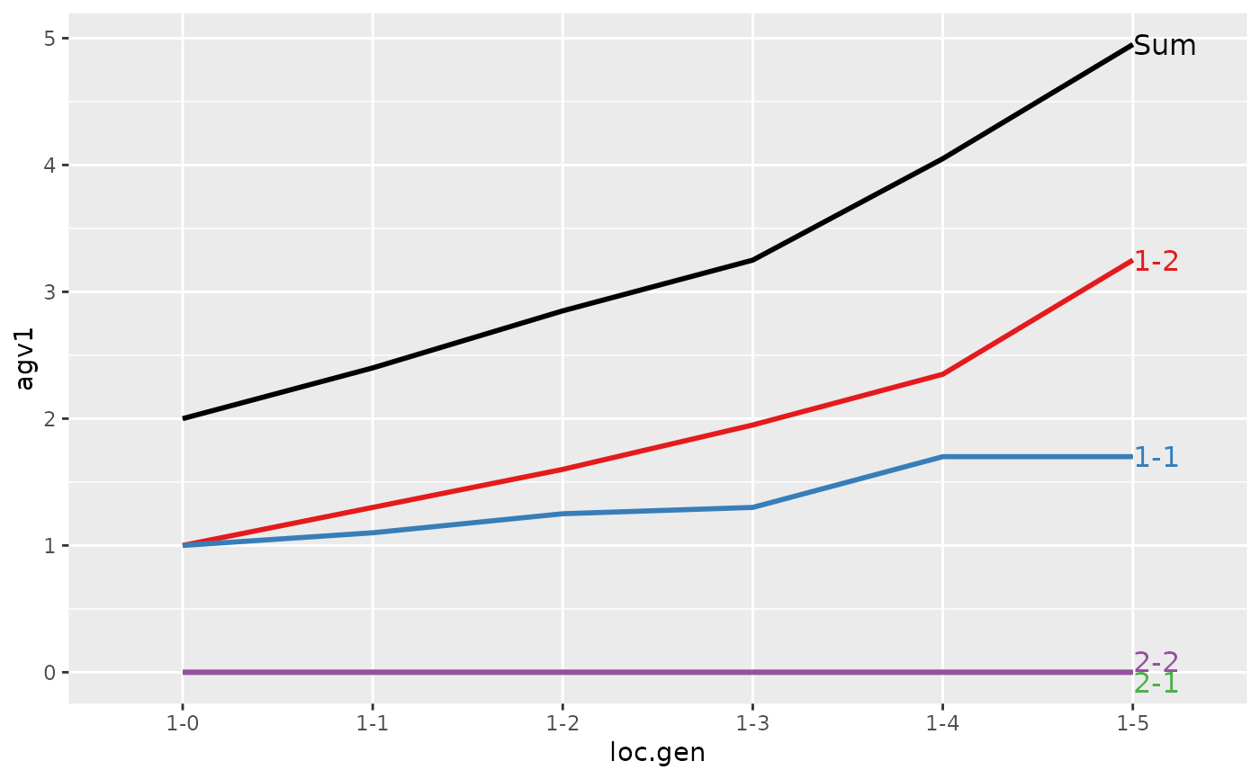
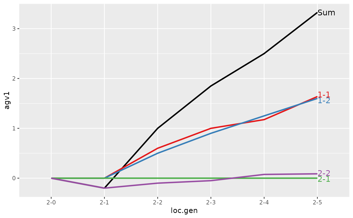
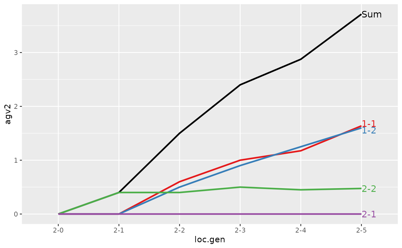
#> > (res <- AlphaPart(x=ped, colPath="loc", colBV=c("agv1", "agv2")))
#>
#> Size:
#> - individuals: 48
#> - traits: 2 (agv1, agv2)
#> - paths: 2 (1, 2)
#> - unknown (missing) values:
#> agv1 agv2
#> 0 0
#>
#>
#> Partitions of breeding values
#> - individuals: 48
#> - paths: 2 (1, 2)
#> - traits: 2 (agv1, agv2)
#>
#> Trait: agv1
#>
#> id fid mid loc gen sex loc.gen agv1 agv1_pa agv1_w agv1_1 agv1_2
#> 1 01 <NA> <NA> 1 0 2 1-0 2 1 1 2 0
#> 2 02 <NA> <NA> 1 0 1 1-0 2 1 1 2 0
#> 3 03 <NA> <NA> 1 0 2 1-0 2 1 1 2 0
#> 4 04 <NA> <NA> 1 0 2 1-0 2 1 1 2 0
#> 5 05 <NA> <NA> 2 0 2 2-0 0 1 -1 0 0
#> 6 06 <NA> <NA> 2 0 1 2-0 0 1 -1 0 0
#> ...
#> id fid mid loc gen sex loc.gen agv1 agv1_pa agv1_w agv1_1 agv1_2
#> 43 53 44 43 1 5 2 1-5 5.3 4.15 1.15 5.30 0.00
#> 44 54 44 43 1 5 2 1-5 4.2 4.15 0.05 4.20 0.00
#> 45 55 44 45 2 5 2 2-5 4.1 3.15 0.95 3.35 0.75
#> 46 56 44 46 2 5 2 2-5 2.7 3.20 -0.50 3.35 -0.65
#> 47 57 44 47 2 5 2 2-5 3.5 3.20 0.30 3.35 0.15
#> 48 58 44 48 2 5 2 2-5 3.8 4.35 -0.55 3.35 0.45
#>
#> Trait: agv2
#>
#> id fid mid loc gen sex loc.gen agv2 agv2_pa agv2_w agv2_1 agv2_2
#> 1 01 <NA> <NA> 1 0 2 1-0 2 1 1 2 0
#> 2 02 <NA> <NA> 1 0 1 1-0 2 1 1 2 0
#> 3 03 <NA> <NA> 1 0 2 1-0 2 1 1 2 0
#> 4 04 <NA> <NA> 1 0 2 1-0 2 1 1 2 0
#> 5 05 <NA> <NA> 2 0 2 2-0 0 1 -1 0 0
#> 6 06 <NA> <NA> 2 0 1 2-0 0 1 -1 0 0
#> ...
#> id fid mid loc gen sex loc.gen agv2 agv2_pa agv2_w agv2_1 agv2_2
#> 43 53 44 43 1 5 2 1-5 5.3 4.15 1.15 5.30 0.00
#> 44 54 44 43 1 5 2 1-5 4.2 4.15 0.05 4.20 0.00
#> 45 55 44 45 2 5 2 2-5 3.7 3.65 0.05 3.35 0.35
#> 46 56 44 46 2 5 2 2-5 5.2 4.00 1.20 3.35 1.85
#> 47 57 44 47 2 5 2 2-5 4.1 3.90 0.20 3.35 0.75
#> 48 58 44 48 2 5 2 2-5 4.3 3.60 0.70 3.35 0.95
#>
#>
#> > ## Summarize whole population
#> > (ret <- summary(res))
#>
#>
#> Summary of partitions of breeding values
#> - paths: 2 (1, 2)
#> - traits: 2 (agv1, agv2)
#>
#> Trait: agv1
#>
#> N <NA> Sum 1 2
#> 1 1 48 2.466667 2.391667 0.075
#>
#> Trait: agv2
#>
#> N <NA> Sum 1 2
#> 1 1 48 2.820833 2.391667 0.4291667
#>
#>
#> > ## Summarize and plot by generation (=trend)
#> > (ret <- summary(res, by="gen"))
#>
#>
#> Summary of partitions of breeding values
#> - paths: 2 (1, 2)
#> - traits: 2 (agv1, agv2)
#>
#> Trait: agv1
#>
#> gen N Sum 1 2
#> 1 0 8 1.0000 1.0000 0.0000
#> 2 1 8 1.4875 1.2125 0.2750
#> 3 2 8 1.8875 2.0500 -0.1625
#> 4 3 8 2.7500 2.6250 0.1250
#> 5 4 8 3.6125 3.4875 0.1250
#> 6 5 8 4.0625 3.9750 0.0875
#>
#> Trait: agv2
#>
#> gen N Sum 1 2
#> 1 0 8 1.0000 1.0000 0.0000
#> 2 1 8 1.5500 1.2125 0.3375
#> 3 2 8 2.7125 2.0500 0.6625
#> 4 3 8 3.2750 2.6250 0.6500
#> 5 4 8 3.9250 3.4875 0.4375
#> 6 5 8 4.4625 3.9750 0.4875
#>
#>
#> > plot(ret)
 #>
#> > ## Summarize and plot location specific trends
#> > (ret <- summary(res, by="loc.gen"))
#>
#>
#> Summary of partitions of breeding values
#> - paths: 2 (1, 2)
#> - traits: 2 (agv1, agv2)
#>
#> Trait: agv1
#>
#> loc.gen N Sum 1 2
#> 1 1-0 4 2.000 2.000 0.000
#> 2 1-1 4 2.425 2.425 0.000
#> 3 1-2 4 2.700 2.700 0.000
#> 4 1-3 4 3.250 3.250 0.000
#> 5 1-4 4 4.275 4.275 0.000
#> 6 1-5 4 4.600 4.600 0.000
#> 7 2-0 4 0.000 0.000 0.000
#> 8 2-1 4 0.550 0.000 0.550
#> 9 2-2 4 1.075 1.400 -0.325
#> 10 2-3 4 2.250 2.000 0.250
#> 11 2-4 4 2.950 2.700 0.250
#> 12 2-5 4 3.525 3.350 0.175
#>
#> Trait: agv2
#>
#> loc.gen N Sum 1 2
#> 1 1-0 4 2.000 2.000 0.000
#> 2 1-1 4 2.425 2.425 0.000
#> 3 1-2 4 2.700 2.700 0.000
#> 4 1-3 4 3.250 3.250 0.000
#> 5 1-4 4 4.275 4.275 0.000
#> 6 1-5 4 4.600 4.600 0.000
#> 7 2-0 4 0.000 0.000 0.000
#> 8 2-1 4 0.675 0.000 0.675
#> 9 2-2 4 2.725 1.400 1.325
#> 10 2-3 4 3.300 2.000 1.300
#> 11 2-4 4 3.575 2.700 0.875
#> 12 2-5 4 4.325 3.350 0.975
#>
#>
#> > plot(ret)
#>
#> > ## Summarize and plot location specific trends
#> > (ret <- summary(res, by="loc.gen"))
#>
#>
#> Summary of partitions of breeding values
#> - paths: 2 (1, 2)
#> - traits: 2 (agv1, agv2)
#>
#> Trait: agv1
#>
#> loc.gen N Sum 1 2
#> 1 1-0 4 2.000 2.000 0.000
#> 2 1-1 4 2.425 2.425 0.000
#> 3 1-2 4 2.700 2.700 0.000
#> 4 1-3 4 3.250 3.250 0.000
#> 5 1-4 4 4.275 4.275 0.000
#> 6 1-5 4 4.600 4.600 0.000
#> 7 2-0 4 0.000 0.000 0.000
#> 8 2-1 4 0.550 0.000 0.550
#> 9 2-2 4 1.075 1.400 -0.325
#> 10 2-3 4 2.250 2.000 0.250
#> 11 2-4 4 2.950 2.700 0.250
#> 12 2-5 4 3.525 3.350 0.175
#>
#> Trait: agv2
#>
#> loc.gen N Sum 1 2
#> 1 1-0 4 2.000 2.000 0.000
#> 2 1-1 4 2.425 2.425 0.000
#> 3 1-2 4 2.700 2.700 0.000
#> 4 1-3 4 3.250 3.250 0.000
#> 5 1-4 4 4.275 4.275 0.000
#> 6 1-5 4 4.600 4.600 0.000
#> 7 2-0 4 0.000 0.000 0.000
#> 8 2-1 4 0.675 0.000 0.675
#> 9 2-2 4 2.725 1.400 1.325
#> 10 2-3 4 3.300 2.000 1.300
#> 11 2-4 4 3.575 2.700 0.875
#> 12 2-5 4 4.325 3.350 0.975
#>
#>
#> > plot(ret)
 #>
#> > ## Summarize and plot location specific trends but only for location 1
#> > (ret <- summary(res, by="loc.gen", subset=res[[1]]$loc == 1))
#>
#>
#> Summary of partitions of breeding values
#> - paths: 2 (1, 2)
#> - traits: 2 (agv1, agv2)
#>
#> Trait: agv1
#>
#> loc.gen N Sum 1 2
#> 1 1-0 4 2.000 2.000 0
#> 2 1-1 4 2.425 2.425 0
#> 3 1-2 4 2.700 2.700 0
#> 4 1-3 4 3.250 3.250 0
#> 5 1-4 4 4.275 4.275 0
#> 6 1-5 4 4.600 4.600 0
#>
#> Trait: agv2
#>
#> loc.gen N Sum 1 2
#> 1 1-0 4 2.000 2.000 0
#> 2 1-1 4 2.425 2.425 0
#> 3 1-2 4 2.700 2.700 0
#> 4 1-3 4 3.250 3.250 0
#> 5 1-4 4 4.275 4.275 0
#> 6 1-5 4 4.600 4.600 0
#>
#>
#> > plot(ret)
#>
#> > ## Summarize and plot location specific trends but only for location 1
#> > (ret <- summary(res, by="loc.gen", subset=res[[1]]$loc == 1))
#>
#>
#> Summary of partitions of breeding values
#> - paths: 2 (1, 2)
#> - traits: 2 (agv1, agv2)
#>
#> Trait: agv1
#>
#> loc.gen N Sum 1 2
#> 1 1-0 4 2.000 2.000 0
#> 2 1-1 4 2.425 2.425 0
#> 3 1-2 4 2.700 2.700 0
#> 4 1-3 4 3.250 3.250 0
#> 5 1-4 4 4.275 4.275 0
#> 6 1-5 4 4.600 4.600 0
#>
#> Trait: agv2
#>
#> loc.gen N Sum 1 2
#> 1 1-0 4 2.000 2.000 0
#> 2 1-1 4 2.425 2.425 0
#> 3 1-2 4 2.700 2.700 0
#> 4 1-3 4 3.250 3.250 0
#> 5 1-4 4 4.275 4.275 0
#> 6 1-5 4 4.600 4.600 0
#>
#>
#> > plot(ret)

 #>
#> > ## Summarize and plot location specific trends but only for location 2
#> > (ret <- summary(res, by="loc.gen", subset=res[[1]]$loc == 2))
#>
#>
#> Summary of partitions of breeding values
#> - paths: 2 (1, 2)
#> - traits: 2 (agv1, agv2)
#>
#> Trait: agv1
#>
#> loc.gen N Sum 1 2
#> 1 2-0 4 0.000 0.00 0.000
#> 2 2-1 4 0.550 0.00 0.550
#> 3 2-2 4 1.075 1.40 -0.325
#> 4 2-3 4 2.250 2.00 0.250
#> 5 2-4 4 2.950 2.70 0.250
#> 6 2-5 4 3.525 3.35 0.175
#>
#> Trait: agv2
#>
#> loc.gen N Sum 1 2
#> 1 2-0 4 0.000 0.00 0.000
#> 2 2-1 4 0.675 0.00 0.675
#> 3 2-2 4 2.725 1.40 1.325
#> 4 2-3 4 3.300 2.00 1.300
#> 5 2-4 4 3.575 2.70 0.875
#> 6 2-5 4 4.325 3.35 0.975
#>
#>
#> > plot(ret)
#>
#> > ## Summarize and plot location specific trends but only for location 2
#> > (ret <- summary(res, by="loc.gen", subset=res[[1]]$loc == 2))
#>
#>
#> Summary of partitions of breeding values
#> - paths: 2 (1, 2)
#> - traits: 2 (agv1, agv2)
#>
#> Trait: agv1
#>
#> loc.gen N Sum 1 2
#> 1 2-0 4 0.000 0.00 0.000
#> 2 2-1 4 0.550 0.00 0.550
#> 3 2-2 4 1.075 1.40 -0.325
#> 4 2-3 4 2.250 2.00 0.250
#> 5 2-4 4 2.950 2.70 0.250
#> 6 2-5 4 3.525 3.35 0.175
#>
#> Trait: agv2
#>
#> loc.gen N Sum 1 2
#> 1 2-0 4 0.000 0.00 0.000
#> 2 2-1 4 0.675 0.00 0.675
#> 3 2-2 4 2.725 1.40 1.325
#> 4 2-3 4 3.300 2.00 1.300
#> 5 2-4 4 3.575 2.70 0.875
#> 6 2-5 4 4.325 3.35 0.975
#>
#>
#> > plot(ret)
 #>
#> > ## Compute partitions by location and sex
#> > ped$loc.sex <- with(ped, paste(loc, sex, sep="-"))
#>
#> > (res <- AlphaPart(x=ped, colPath="loc.sex", colBV=c("agv1", "agv2")))
#>
#> Size:
#> - individuals: 48
#> - traits: 2 (agv1, agv2)
#> - paths: 4 (1-1, 1-2, 2-1, 2-2)
#> - unknown (missing) values:
#> agv1 agv2
#> 0 0
#>
#>
#> Partitions of breeding values
#> - individuals: 48
#> - paths: 4 (1-1, 1-2, 2-1, 2-2)
#> - traits: 2 (agv1, agv2)
#>
#> Trait: agv1
#>
#> id fid mid loc gen sex loc.gen loc.sex agv1 agv1_pa agv1_w agv1_1-1 agv1_1-2 agv1_2-1 agv1_2-2
#> 1 01 <NA> <NA> 1 0 2 1-0 1-2 2 1 1 0 2 0 0
#> 2 02 <NA> <NA> 1 0 1 1-0 1-1 2 1 1 2 0 0 0
#> 3 03 <NA> <NA> 1 0 2 1-0 1-2 2 1 1 0 2 0 0
#> 4 04 <NA> <NA> 1 0 2 1-0 1-2 2 1 1 0 2 0 0
#> 5 05 <NA> <NA> 2 0 2 2-0 2-2 0 1 -1 0 0 0 0
#> 6 06 <NA> <NA> 2 0 1 2-0 2-1 0 1 -1 0 0 0 0
#> ...
#> id fid mid loc gen sex loc.gen loc.sex agv1 agv1_pa agv1_w agv1_1-1 agv1_1-2 agv1_2-1 agv1_2-2
#> 43 53 44 43 1 5 2 1-5 1-2 5.3 4.15 1.15 2.3250 2.9750 0 0.00
#> 44 54 44 43 1 5 2 1-5 1-2 4.2 4.15 0.05 2.3250 1.8750 0 0.00
#> 45 55 44 45 2 5 2 2-5 2-2 4.1 3.15 0.95 2.2625 1.0875 0 0.75
#> 46 56 44 46 2 5 2 2-5 2-2 2.7 3.20 -0.50 2.2625 1.0875 0 -0.65
#> 47 57 44 47 2 5 2 2-5 2-2 3.5 3.20 0.30 2.2625 1.0875 0 0.15
#> 48 58 44 48 2 5 2 2-5 2-2 3.8 4.35 -0.55 2.2625 1.0875 0 0.45
#>
#> Trait: agv2
#>
#> id fid mid loc gen sex loc.gen loc.sex agv2 agv2_pa agv2_w agv2_1-1 agv2_1-2 agv2_2-1 agv2_2-2
#> 1 01 <NA> <NA> 1 0 2 1-0 1-2 2 1 1 0 2 0 0
#> 2 02 <NA> <NA> 1 0 1 1-0 1-1 2 1 1 2 0 0 0
#> 3 03 <NA> <NA> 1 0 2 1-0 1-2 2 1 1 0 2 0 0
#> 4 04 <NA> <NA> 1 0 2 1-0 1-2 2 1 1 0 2 0 0
#> 5 05 <NA> <NA> 2 0 2 2-0 2-2 0 1 -1 0 0 0 0
#> 6 06 <NA> <NA> 2 0 1 2-0 2-1 0 1 -1 0 0 0 0
#> ...
#> id fid mid loc gen sex loc.gen loc.sex agv2 agv2_pa agv2_w agv2_1-1 agv2_1-2 agv2_2-1 agv2_2-2
#> 43 53 44 43 1 5 2 1-5 1-2 5.3 4.15 1.15 2.3250 2.9750 0 0.00
#> 44 54 44 43 1 5 2 1-5 1-2 4.2 4.15 0.05 2.3250 1.8750 0 0.00
#> 45 55 44 45 2 5 2 2-5 2-2 3.7 3.65 0.05 2.2625 1.0875 0 0.35
#> 46 56 44 46 2 5 2 2-5 2-2 5.2 4.00 1.20 2.2625 1.0875 0 1.85
#> 47 57 44 47 2 5 2 2-5 2-2 4.1 3.90 0.20 2.2625 1.0875 0 0.75
#> 48 58 44 48 2 5 2 2-5 2-2 4.3 3.60 0.70 2.2625 1.0875 0 0.95
#>
#>
#> > ## Summarize and plot by generation (=trend)
#> > (ret <- summary(res, by="gen"))
#>
#>
#> Summary of partitions of breeding values
#> - paths: 4 (1-1, 1-2, 2-1, 2-2)
#> - traits: 2 (agv1, agv2)
#>
#> Trait: agv1
#>
#> gen N Sum 1-1 1-2 2-1 2-2
#> 1 0 8 1.0000 0.25000 0.75000 0 0.0000
#> 2 1 8 1.4875 0.60000 0.61250 0 0.2750
#> 3 2 8 1.8875 1.16875 0.88125 0 -0.1625
#> 4 3 8 2.7500 1.45000 1.17500 0 0.1250
#> 5 4 8 3.6125 1.92500 1.56250 0 0.1250
#> 6 5 8 4.0625 2.29375 1.68125 0 0.0875
#>
#> Trait: agv2
#>
#> gen N Sum 1-1 1-2 2-1 2-2
#> 1 0 8 1.0000 0.25000 0.75000 0 0.0000
#> 2 1 8 1.5500 0.60000 0.61250 0 0.3375
#> 3 2 8 2.7125 1.16875 0.88125 0 0.6625
#> 4 3 8 3.2750 1.45000 1.17500 0 0.6500
#> 5 4 8 3.9250 1.92500 1.56250 0 0.4375
#> 6 5 8 4.4625 2.29375 1.68125 0 0.4875
#>
#>
#> > plot(ret)
#>
#> > ## Compute partitions by location and sex
#> > ped$loc.sex <- with(ped, paste(loc, sex, sep="-"))
#>
#> > (res <- AlphaPart(x=ped, colPath="loc.sex", colBV=c("agv1", "agv2")))
#>
#> Size:
#> - individuals: 48
#> - traits: 2 (agv1, agv2)
#> - paths: 4 (1-1, 1-2, 2-1, 2-2)
#> - unknown (missing) values:
#> agv1 agv2
#> 0 0
#>
#>
#> Partitions of breeding values
#> - individuals: 48
#> - paths: 4 (1-1, 1-2, 2-1, 2-2)
#> - traits: 2 (agv1, agv2)
#>
#> Trait: agv1
#>
#> id fid mid loc gen sex loc.gen loc.sex agv1 agv1_pa agv1_w agv1_1-1 agv1_1-2 agv1_2-1 agv1_2-2
#> 1 01 <NA> <NA> 1 0 2 1-0 1-2 2 1 1 0 2 0 0
#> 2 02 <NA> <NA> 1 0 1 1-0 1-1 2 1 1 2 0 0 0
#> 3 03 <NA> <NA> 1 0 2 1-0 1-2 2 1 1 0 2 0 0
#> 4 04 <NA> <NA> 1 0 2 1-0 1-2 2 1 1 0 2 0 0
#> 5 05 <NA> <NA> 2 0 2 2-0 2-2 0 1 -1 0 0 0 0
#> 6 06 <NA> <NA> 2 0 1 2-0 2-1 0 1 -1 0 0 0 0
#> ...
#> id fid mid loc gen sex loc.gen loc.sex agv1 agv1_pa agv1_w agv1_1-1 agv1_1-2 agv1_2-1 agv1_2-2
#> 43 53 44 43 1 5 2 1-5 1-2 5.3 4.15 1.15 2.3250 2.9750 0 0.00
#> 44 54 44 43 1 5 2 1-5 1-2 4.2 4.15 0.05 2.3250 1.8750 0 0.00
#> 45 55 44 45 2 5 2 2-5 2-2 4.1 3.15 0.95 2.2625 1.0875 0 0.75
#> 46 56 44 46 2 5 2 2-5 2-2 2.7 3.20 -0.50 2.2625 1.0875 0 -0.65
#> 47 57 44 47 2 5 2 2-5 2-2 3.5 3.20 0.30 2.2625 1.0875 0 0.15
#> 48 58 44 48 2 5 2 2-5 2-2 3.8 4.35 -0.55 2.2625 1.0875 0 0.45
#>
#> Trait: agv2
#>
#> id fid mid loc gen sex loc.gen loc.sex agv2 agv2_pa agv2_w agv2_1-1 agv2_1-2 agv2_2-1 agv2_2-2
#> 1 01 <NA> <NA> 1 0 2 1-0 1-2 2 1 1 0 2 0 0
#> 2 02 <NA> <NA> 1 0 1 1-0 1-1 2 1 1 2 0 0 0
#> 3 03 <NA> <NA> 1 0 2 1-0 1-2 2 1 1 0 2 0 0
#> 4 04 <NA> <NA> 1 0 2 1-0 1-2 2 1 1 0 2 0 0
#> 5 05 <NA> <NA> 2 0 2 2-0 2-2 0 1 -1 0 0 0 0
#> 6 06 <NA> <NA> 2 0 1 2-0 2-1 0 1 -1 0 0 0 0
#> ...
#> id fid mid loc gen sex loc.gen loc.sex agv2 agv2_pa agv2_w agv2_1-1 agv2_1-2 agv2_2-1 agv2_2-2
#> 43 53 44 43 1 5 2 1-5 1-2 5.3 4.15 1.15 2.3250 2.9750 0 0.00
#> 44 54 44 43 1 5 2 1-5 1-2 4.2 4.15 0.05 2.3250 1.8750 0 0.00
#> 45 55 44 45 2 5 2 2-5 2-2 3.7 3.65 0.05 2.2625 1.0875 0 0.35
#> 46 56 44 46 2 5 2 2-5 2-2 5.2 4.00 1.20 2.2625 1.0875 0 1.85
#> 47 57 44 47 2 5 2 2-5 2-2 4.1 3.90 0.20 2.2625 1.0875 0 0.75
#> 48 58 44 48 2 5 2 2-5 2-2 4.3 3.60 0.70 2.2625 1.0875 0 0.95
#>
#>
#> > ## Summarize and plot by generation (=trend)
#> > (ret <- summary(res, by="gen"))
#>
#>
#> Summary of partitions of breeding values
#> - paths: 4 (1-1, 1-2, 2-1, 2-2)
#> - traits: 2 (agv1, agv2)
#>
#> Trait: agv1
#>
#> gen N Sum 1-1 1-2 2-1 2-2
#> 1 0 8 1.0000 0.25000 0.75000 0 0.0000
#> 2 1 8 1.4875 0.60000 0.61250 0 0.2750
#> 3 2 8 1.8875 1.16875 0.88125 0 -0.1625
#> 4 3 8 2.7500 1.45000 1.17500 0 0.1250
#> 5 4 8 3.6125 1.92500 1.56250 0 0.1250
#> 6 5 8 4.0625 2.29375 1.68125 0 0.0875
#>
#> Trait: agv2
#>
#> gen N Sum 1-1 1-2 2-1 2-2
#> 1 0 8 1.0000 0.25000 0.75000 0 0.0000
#> 2 1 8 1.5500 0.60000 0.61250 0 0.3375
#> 3 2 8 2.7125 1.16875 0.88125 0 0.6625
#> 4 3 8 3.2750 1.45000 1.17500 0 0.6500
#> 5 4 8 3.9250 1.92500 1.56250 0 0.4375
#> 6 5 8 4.4625 2.29375 1.68125 0 0.4875
#>
#>
#> > plot(ret)
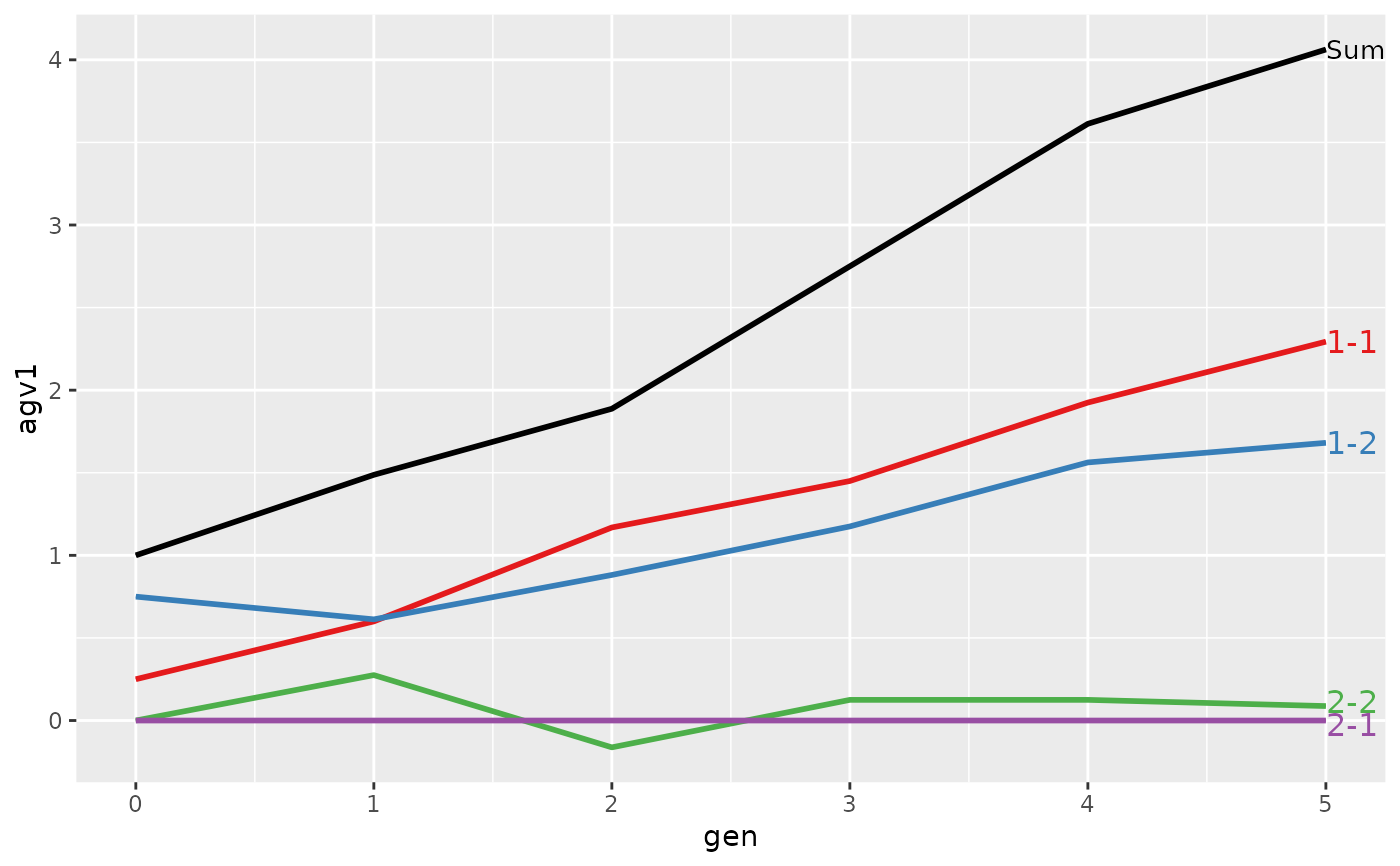
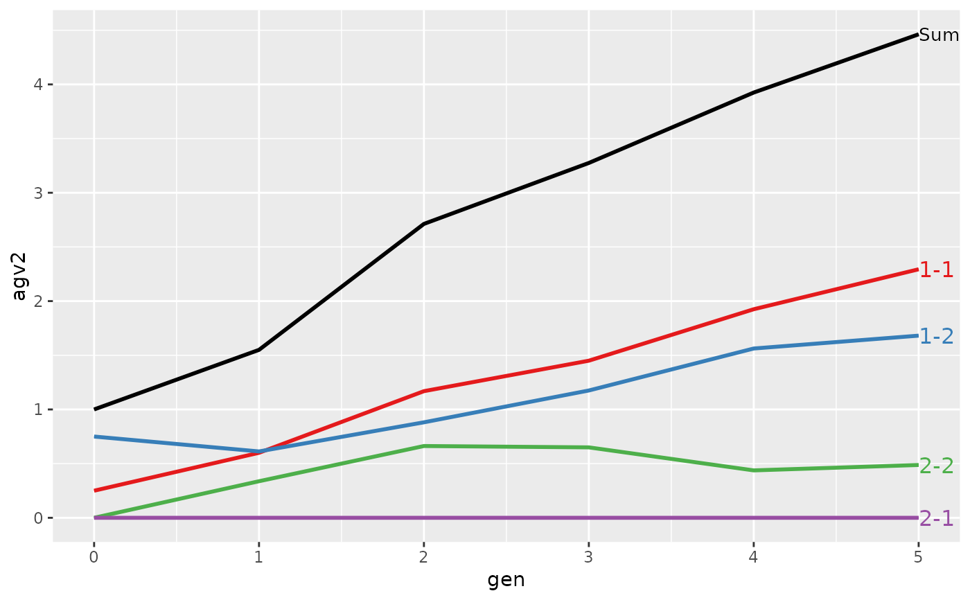 #>
#> > plot(ret, lineTypeList=list("-1"=1, "-2"=2, def=3))
#>
#> > plot(ret, lineTypeList=list("-1"=1, "-2"=2, def=3))
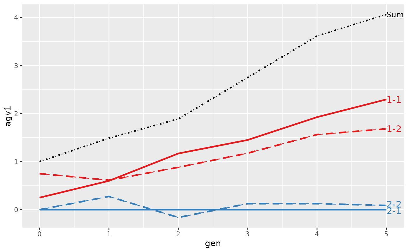
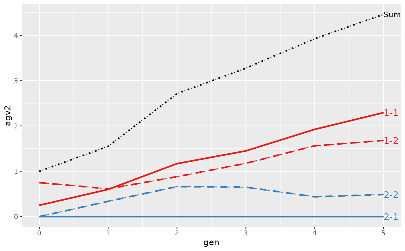 #>
#> > ## Summarize and plot location specific trends
#> > (ret <- summary(res, by="loc.gen"))
#>
#>
#> Summary of partitions of breeding values
#> - paths: 4 (1-1, 1-2, 2-1, 2-2)
#> - traits: 2 (agv1, agv2)
#>
#> Trait: agv1
#>
#> loc.gen N Sum 1-1 1-2 2-1 2-2
#> 1 1-0 4 2.000 0.5000 1.5000 0 0.000
#> 2 1-1 4 2.425 1.2000 1.2250 0 0.000
#> 3 1-2 4 2.700 1.4375 1.2625 0 0.000
#> 4 1-3 4 3.250 1.6750 1.5750 0 0.000
#> 5 1-4 4 4.275 2.1000 2.1750 0 0.000
#> 6 1-5 4 4.600 2.3250 2.2750 0 0.000
#> 7 2-0 4 0.000 0.0000 0.0000 0 0.000
#> 8 2-1 4 0.550 0.0000 0.0000 0 0.550
#> 9 2-2 4 1.075 0.9000 0.5000 0 -0.325
#> 10 2-3 4 2.250 1.2250 0.7750 0 0.250
#> 11 2-4 4 2.950 1.7500 0.9500 0 0.250
#> 12 2-5 4 3.525 2.2625 1.0875 0 0.175
#>
#> Trait: agv2
#>
#> loc.gen N Sum 1-1 1-2 2-1 2-2
#> 1 1-0 4 2.000 0.5000 1.5000 0 0.000
#> 2 1-1 4 2.425 1.2000 1.2250 0 0.000
#> 3 1-2 4 2.700 1.4375 1.2625 0 0.000
#> 4 1-3 4 3.250 1.6750 1.5750 0 0.000
#> 5 1-4 4 4.275 2.1000 2.1750 0 0.000
#> 6 1-5 4 4.600 2.3250 2.2750 0 0.000
#> 7 2-0 4 0.000 0.0000 0.0000 0 0.000
#> 8 2-1 4 0.675 0.0000 0.0000 0 0.675
#> 9 2-2 4 2.725 0.9000 0.5000 0 1.325
#> 10 2-3 4 3.300 1.2250 0.7750 0 1.300
#> 11 2-4 4 3.575 1.7500 0.9500 0 0.875
#> 12 2-5 4 4.325 2.2625 1.0875 0 0.975
#>
#>
#> > plot(ret, lineTypeList=list("-1"=1, "-2"=2, def=3))
#>
#> > ## Summarize and plot location specific trends
#> > (ret <- summary(res, by="loc.gen"))
#>
#>
#> Summary of partitions of breeding values
#> - paths: 4 (1-1, 1-2, 2-1, 2-2)
#> - traits: 2 (agv1, agv2)
#>
#> Trait: agv1
#>
#> loc.gen N Sum 1-1 1-2 2-1 2-2
#> 1 1-0 4 2.000 0.5000 1.5000 0 0.000
#> 2 1-1 4 2.425 1.2000 1.2250 0 0.000
#> 3 1-2 4 2.700 1.4375 1.2625 0 0.000
#> 4 1-3 4 3.250 1.6750 1.5750 0 0.000
#> 5 1-4 4 4.275 2.1000 2.1750 0 0.000
#> 6 1-5 4 4.600 2.3250 2.2750 0 0.000
#> 7 2-0 4 0.000 0.0000 0.0000 0 0.000
#> 8 2-1 4 0.550 0.0000 0.0000 0 0.550
#> 9 2-2 4 1.075 0.9000 0.5000 0 -0.325
#> 10 2-3 4 2.250 1.2250 0.7750 0 0.250
#> 11 2-4 4 2.950 1.7500 0.9500 0 0.250
#> 12 2-5 4 3.525 2.2625 1.0875 0 0.175
#>
#> Trait: agv2
#>
#> loc.gen N Sum 1-1 1-2 2-1 2-2
#> 1 1-0 4 2.000 0.5000 1.5000 0 0.000
#> 2 1-1 4 2.425 1.2000 1.2250 0 0.000
#> 3 1-2 4 2.700 1.4375 1.2625 0 0.000
#> 4 1-3 4 3.250 1.6750 1.5750 0 0.000
#> 5 1-4 4 4.275 2.1000 2.1750 0 0.000
#> 6 1-5 4 4.600 2.3250 2.2750 0 0.000
#> 7 2-0 4 0.000 0.0000 0.0000 0 0.000
#> 8 2-1 4 0.675 0.0000 0.0000 0 0.675
#> 9 2-2 4 2.725 0.9000 0.5000 0 1.325
#> 10 2-3 4 3.300 1.2250 0.7750 0 1.300
#> 11 2-4 4 3.575 1.7500 0.9500 0 0.875
#> 12 2-5 4 4.325 2.2625 1.0875 0 0.975
#>
#>
#> > plot(ret, lineTypeList=list("-1"=1, "-2"=2, def=3))
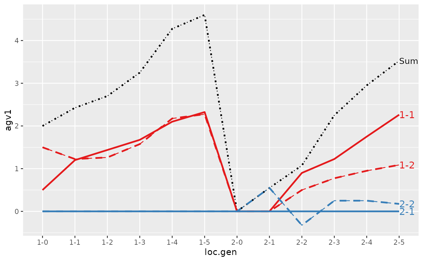
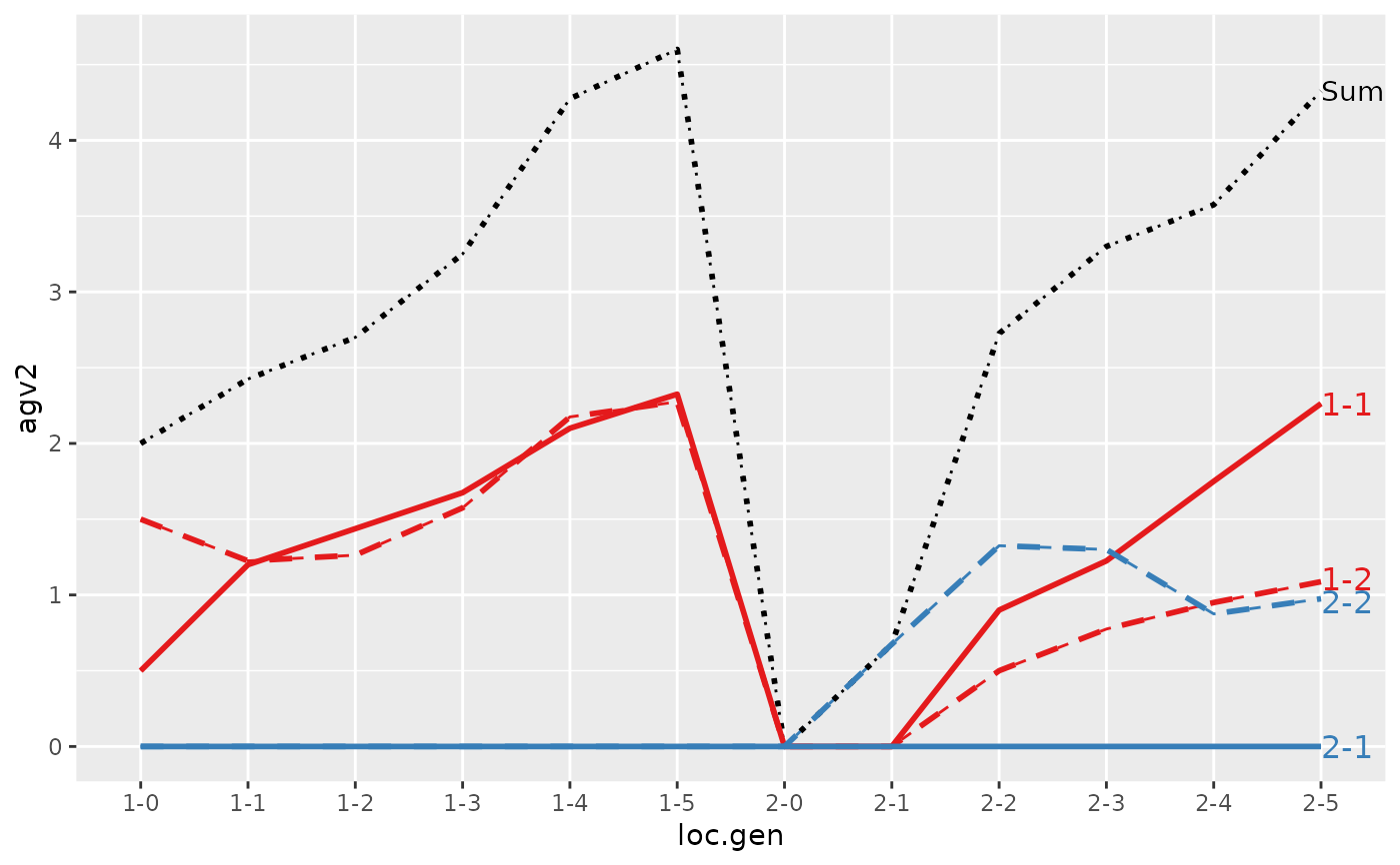 #>
#> > ## Summarize and plot location specific trends but only for location 1
#> > (ret <- summary(res, by="loc.gen", subset=res[[1]]$loc == 1))
#>
#>
#> Summary of partitions of breeding values
#> - paths: 4 (1-1, 1-2, 2-1, 2-2)
#> - traits: 2 (agv1, agv2)
#>
#> Trait: agv1
#>
#> loc.gen N Sum 1-1 1-2 2-1 2-2
#> 1 1-0 4 2.000 0.5000 1.5000 0 0
#> 2 1-1 4 2.425 1.2000 1.2250 0 0
#> 3 1-2 4 2.700 1.4375 1.2625 0 0
#> 4 1-3 4 3.250 1.6750 1.5750 0 0
#> 5 1-4 4 4.275 2.1000 2.1750 0 0
#> 6 1-5 4 4.600 2.3250 2.2750 0 0
#>
#> Trait: agv2
#>
#> loc.gen N Sum 1-1 1-2 2-1 2-2
#> 1 1-0 4 2.000 0.5000 1.5000 0 0
#> 2 1-1 4 2.425 1.2000 1.2250 0 0
#> 3 1-2 4 2.700 1.4375 1.2625 0 0
#> 4 1-3 4 3.250 1.6750 1.5750 0 0
#> 5 1-4 4 4.275 2.1000 2.1750 0 0
#> 6 1-5 4 4.600 2.3250 2.2750 0 0
#>
#>
#> > plot(ret)
#>
#> > ## Summarize and plot location specific trends but only for location 1
#> > (ret <- summary(res, by="loc.gen", subset=res[[1]]$loc == 1))
#>
#>
#> Summary of partitions of breeding values
#> - paths: 4 (1-1, 1-2, 2-1, 2-2)
#> - traits: 2 (agv1, agv2)
#>
#> Trait: agv1
#>
#> loc.gen N Sum 1-1 1-2 2-1 2-2
#> 1 1-0 4 2.000 0.5000 1.5000 0 0
#> 2 1-1 4 2.425 1.2000 1.2250 0 0
#> 3 1-2 4 2.700 1.4375 1.2625 0 0
#> 4 1-3 4 3.250 1.6750 1.5750 0 0
#> 5 1-4 4 4.275 2.1000 2.1750 0 0
#> 6 1-5 4 4.600 2.3250 2.2750 0 0
#>
#> Trait: agv2
#>
#> loc.gen N Sum 1-1 1-2 2-1 2-2
#> 1 1-0 4 2.000 0.5000 1.5000 0 0
#> 2 1-1 4 2.425 1.2000 1.2250 0 0
#> 3 1-2 4 2.700 1.4375 1.2625 0 0
#> 4 1-3 4 3.250 1.6750 1.5750 0 0
#> 5 1-4 4 4.275 2.1000 2.1750 0 0
#> 6 1-5 4 4.600 2.3250 2.2750 0 0
#>
#>
#> > plot(ret)

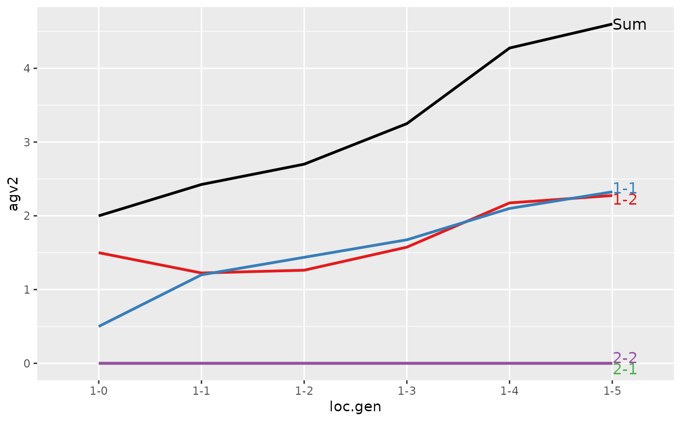 #>
#> > ## Summarize and plot location specific trends but only for location 2
#> > (ret <- summary(res, by="loc.gen", subset=res[[1]]$loc == 2))
#>
#>
#> Summary of partitions of breeding values
#> - paths: 4 (1-1, 1-2, 2-1, 2-2)
#> - traits: 2 (agv1, agv2)
#>
#> Trait: agv1
#>
#> loc.gen N Sum 1-1 1-2 2-1 2-2
#> 1 2-0 4 0.000 0.0000 0.0000 0 0.000
#> 2 2-1 4 0.550 0.0000 0.0000 0 0.550
#> 3 2-2 4 1.075 0.9000 0.5000 0 -0.325
#> 4 2-3 4 2.250 1.2250 0.7750 0 0.250
#> 5 2-4 4 2.950 1.7500 0.9500 0 0.250
#> 6 2-5 4 3.525 2.2625 1.0875 0 0.175
#>
#> Trait: agv2
#>
#> loc.gen N Sum 1-1 1-2 2-1 2-2
#> 1 2-0 4 0.000 0.0000 0.0000 0 0.000
#> 2 2-1 4 0.675 0.0000 0.0000 0 0.675
#> 3 2-2 4 2.725 0.9000 0.5000 0 1.325
#> 4 2-3 4 3.300 1.2250 0.7750 0 1.300
#> 5 2-4 4 3.575 1.7500 0.9500 0 0.875
#> 6 2-5 4 4.325 2.2625 1.0875 0 0.975
#>
#>
#> > plot(ret)
#>
#> > ## Summarize and plot location specific trends but only for location 2
#> > (ret <- summary(res, by="loc.gen", subset=res[[1]]$loc == 2))
#>
#>
#> Summary of partitions of breeding values
#> - paths: 4 (1-1, 1-2, 2-1, 2-2)
#> - traits: 2 (agv1, agv2)
#>
#> Trait: agv1
#>
#> loc.gen N Sum 1-1 1-2 2-1 2-2
#> 1 2-0 4 0.000 0.0000 0.0000 0 0.000
#> 2 2-1 4 0.550 0.0000 0.0000 0 0.550
#> 3 2-2 4 1.075 0.9000 0.5000 0 -0.325
#> 4 2-3 4 2.250 1.2250 0.7750 0 0.250
#> 5 2-4 4 2.950 1.7500 0.9500 0 0.250
#> 6 2-5 4 3.525 2.2625 1.0875 0 0.175
#>
#> Trait: agv2
#>
#> loc.gen N Sum 1-1 1-2 2-1 2-2
#> 1 2-0 4 0.000 0.0000 0.0000 0 0.000
#> 2 2-1 4 0.675 0.0000 0.0000 0 0.675
#> 3 2-2 4 2.725 0.9000 0.5000 0 1.325
#> 4 2-3 4 3.300 1.2250 0.7750 0 1.300
#> 5 2-4 4 3.575 1.7500 0.9500 0 0.875
#> 6 2-5 4 4.325 2.2625 1.0875 0 0.975
#>
#>
#> > plot(ret)
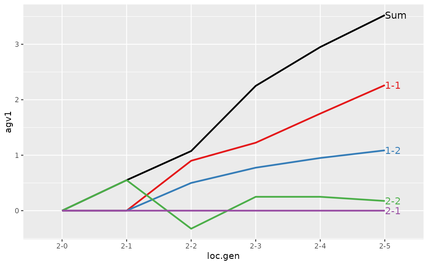
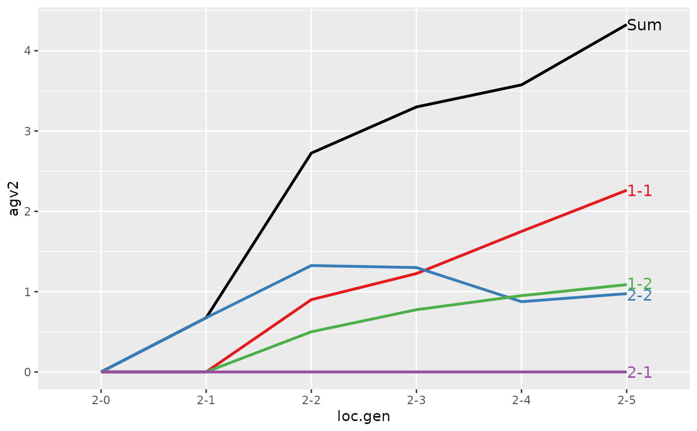 #>
#> > ###-----------------------------------------------------------------------------
#> > ### demo_stohastic.R ends here
# }
#>
#> > ###-----------------------------------------------------------------------------
#> > ### demo_stohastic.R ends here
# }