A function to plot summary of partitioned breeding values.
plot.summaryAlphaPart.RdA function to plot summary of partitioned breeding values.
Usage
# S3 method for class 'summaryAlphaPart'
plot(x, by, sortValue,
  sortValueFUN, sortValueDec, addSum, paths, xlab, ylab, xlim, ylim,
  color, lineSize, lineType, lineTypeList, useDirectLabels, method,
  labelPath, ...)
Arguments
- x
summaryAlphaPart, object from the
AlphaPart(...)orsummary(AlphaPart(...), ...)call.- by
Character, the name of a column by which summary function FUN should be applied; if
NULL(default) summary is given for the whole table.- sortValue
Logical, affect legend attributes via sort of paths according to
sortValueFUNfunction; if not logical, then ordered paths are given as a character vector.- sortValueFUN
Function, that produces single value for one vector, say
meanorsum.- sortValueDec
Logical, sort decreasing.
- addSum
Logical, plot the overall trend.
- paths
Character or list or characters, name of paths to plot; if
NULLplot all paths; see examples.- xlab
Character, x-axis label.
- ylab
Character, y-axis label; can be a vector of several labels if there are more traits in
x(recycled!).- xlim
Numeric, a vector of two values with x-axis limits; use a list of vectors for more traits.
- ylim
Numeric, a vector of two values with y-axis limits; use a list of vectors for more traits.
- color
Character, color names; by default a set of 54 colors is predefined from the RColorBrewer package; in addition a black colour is attached at the begining for the overall trend; if there are more paths than colors then recycling occours.
- lineSize
Numeric, line width.
- lineType
Numeric, line type (recycled); can be used only if lineTypeList=NULL.
- lineTypeList
List, named list of numeric values that help to point out a set of paths (distinguished with line type) within upper level of paths (distinguished by, color), e.g., lineTypeList=list("-1"=1, "-2"=2, def=1) will lead to use of line 2, for paths having "-2" at the end of path name, while line type 1 (default) will, be used for other paths; specification of this argument also causes recycling of colors for the upper level of paths; if NULL all lines have a standard line type, otherwise
lineTypedoes not have any effect.- useDirectLabels
Logical, use directlabels package for legend.
- method
List, method for direct.label.
- labelPath
Character, legend title; used only if
useDirectLabels=FALSE.- ...
Arguments passed to other functions (not used at the moment).
Value
A list of ggplot objects that can be further modified or
displayed. For each trait in x there is one plot
visualising summarized values.
Details
Information in summaries of partitions of breeding values can be overhelming due to a large volume of numbers. Plot method can be used to visualise this data in eye pleasing way using ggplot2 graphics.
Examples
# \donttest{
## Partition additive genetic values by country
(res <- AlphaPart(x=AlphaPart.ped, colPath="country", colBV=c("bv1", "bv2")))
#>
#> Size:
#> - individuals: 8
#> - traits: 2 (bv1, bv2)
#> - paths: 2 (domestic, import)
#> - unknown (missing) values:
#> bv1 bv2
#> 0 0
#>
#>
#> Partitions of breeding values
#> - individuals: 8
#> - paths: 2 (domestic, import)
#> - traits: 2 (bv1, bv2)
#>
#> Trait: bv1
#>
#> IId FId MId gen country gender bv1 bv1_pa bv1_w bv1_domestic bv1_import
#> 1 A 1 domestic F 100 104.3333 -4.3333333 100.000 0.000
#> 2 B 1 import M 105 104.3333 0.6666667 0.000 105.000
#> 3 C B A 2 domestic F 104 102.5000 1.5000000 51.500 52.500
#> 4 T B 2 import F 102 52.5000 49.5000000 0.000 102.000
#> 5 D 2 import M 108 104.3333 3.6666667 0.000 108.000
#> 6 E D C 3 domestic M 107 106.0000 1.0000000 26.750 80.250
#> 7 U D 3 import F 107 54.0000 53.0000000 0.000 107.000
#> 8 V E 4 domestic F 109 53.5000 55.5000000 68.875 40.125
#>
#> Trait: bv2
#>
#> IId FId MId gen country gender bv2 bv2_pa bv2_w bv2_domestic bv2_import
#> 1 A 1 domestic F 88 99.66667 -11.666667 88 0
#> 2 B 1 import M 110 99.66667 10.333333 0 110
#> 3 C B A 2 domestic F 100 99.00000 1.000000 45 55
#> 4 T B 2 import F 97 55.00000 42.000000 0 97
#> 5 D 2 import M 101 99.66667 1.333333 0 101
#> 6 E D C 3 domestic M 80 100.50000 -20.500000 2 78
#> 7 U D 3 import F 102 50.50000 51.500000 0 102
#> 8 V E 4 domestic F 105 40.00000 65.000000 66 39
#>
## Summarize population by generation (=trend)
(ret <- summary(res, by="gen"))
#>
#>
#> Summary of partitions of breeding values
#> - paths: 2 (domestic, import)
#> - traits: 2 (bv1, bv2)
#>
#> Trait: bv1
#>
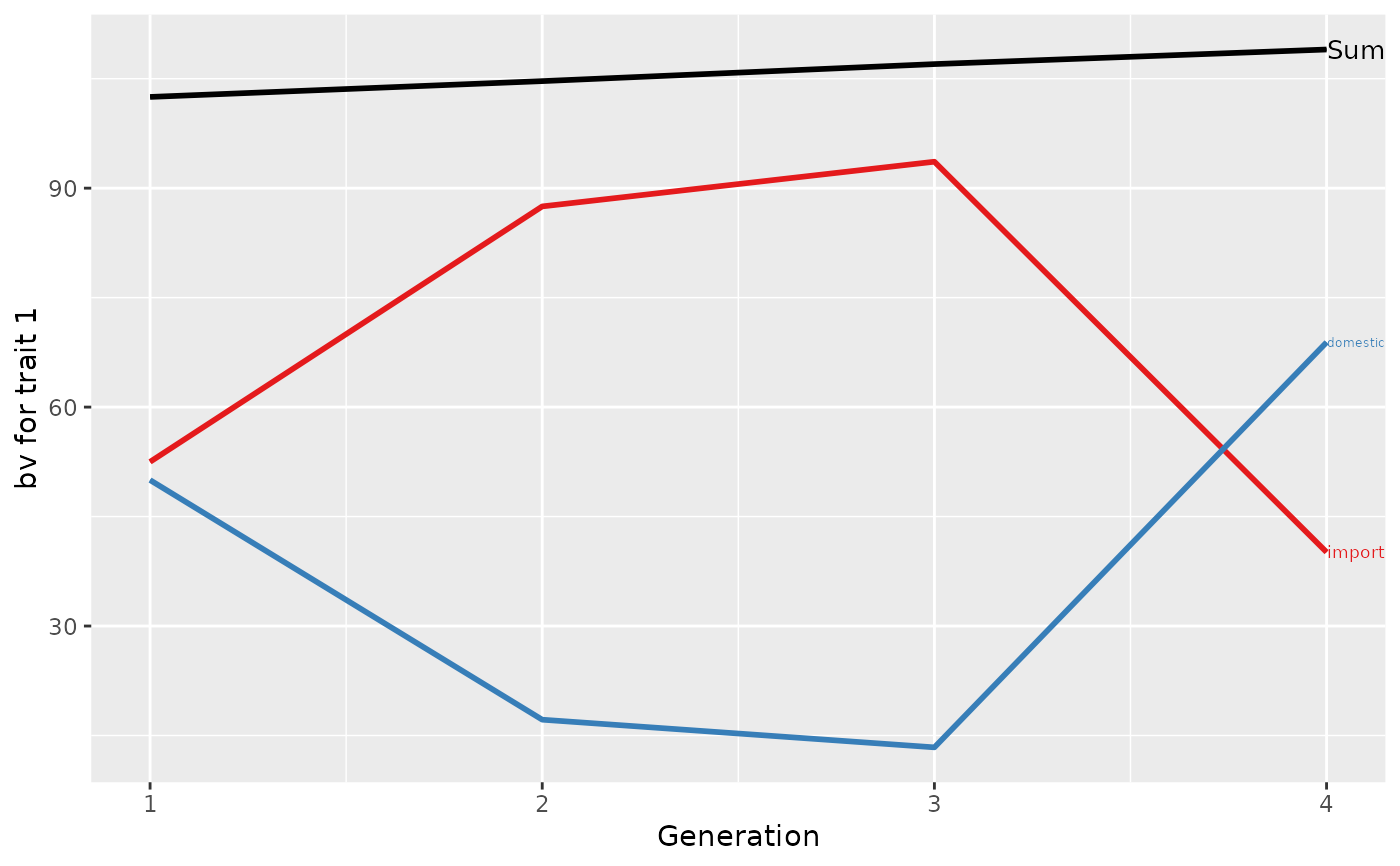
#> gen N Sum domestic import
#> 1 1 2 102.5000 50.00000 52.500
#> 2 2 3 104.6667 17.16667 87.500
#> 3 3 2 107.0000 13.37500 93.625
#> 4 4 1 109.0000 68.87500 40.125
#>
#> Trait: bv2
#>
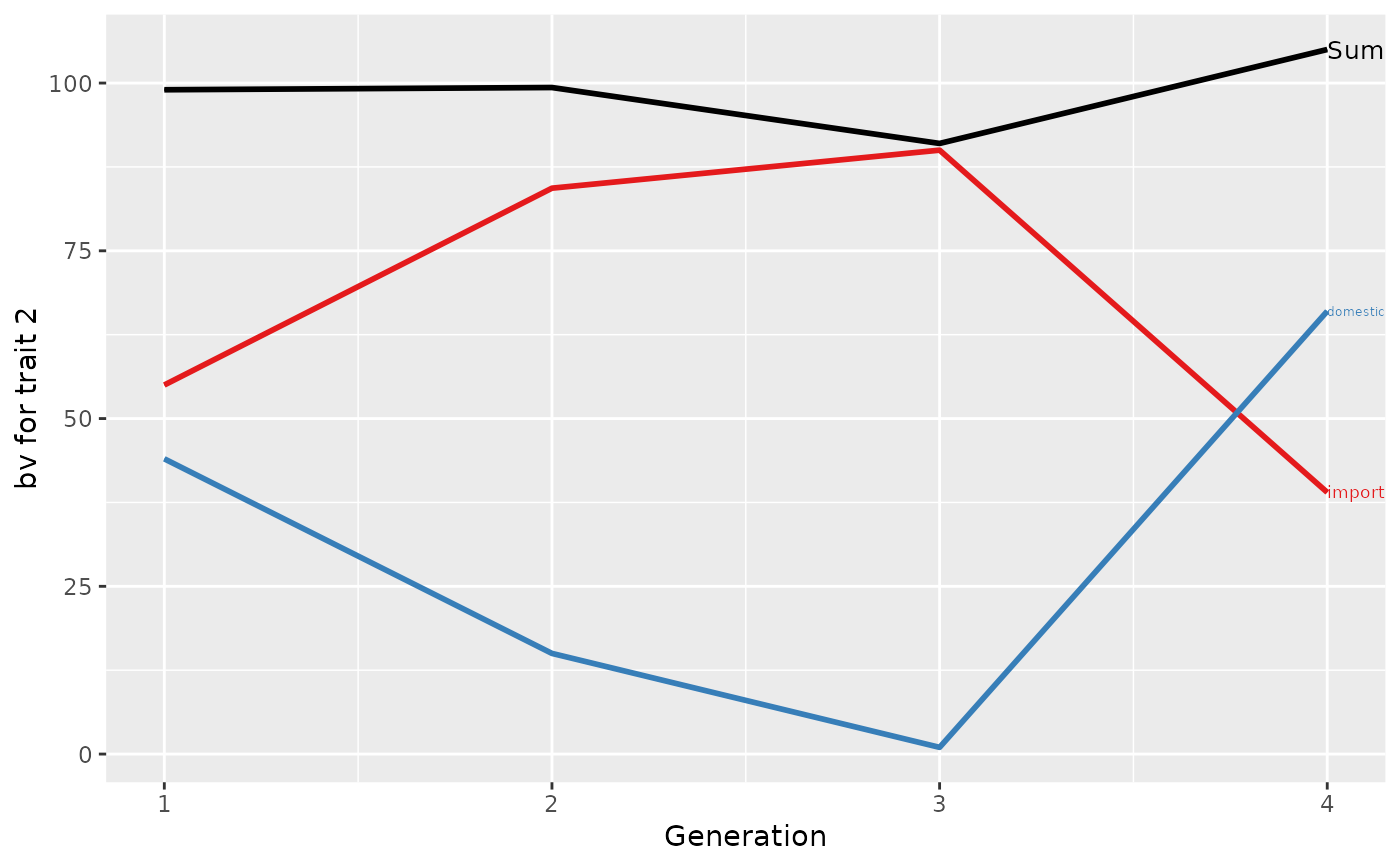
#> gen N Sum domestic import
#> 1 1 2 99.00000 44 55.00000
#> 2 2 3 99.33333 15 84.33333
#> 3 3 2 91.00000 1 90.00000
#> 4 4 1 105.00000 66 39.00000
#>
## Plot the partitions
p <- plot(ret, ylab=c("bv for trait 1", "bv for trait 2"), xlab="Generation")
print(p[[1]]$abs)
#> NULL
print(p[[2]]$abs)
#> NULL
print(p)
 ## Partition additive genetic values by country and sex
AlphaPart.ped$country.gender <- with(AlphaPart.ped, paste(country, gender, sep="-"))
(res <- AlphaPart(x=AlphaPart.ped, colPath="country.gender", colBV=c("bv1", "bv2")))
#>
#> Size:
#> - individuals: 8
#> - traits: 2 (bv1, bv2)
#> - paths: 4 (domestic-F, domestic-M, import-F, import-M)
#> - unknown (missing) values:
#> bv1 bv2
#> 0 0
#>
#>
#> Partitions of breeding values
#> - individuals: 8
#> - paths: 4 (domestic-F, domestic-M, import-F, import-M)
#> - traits: 2 (bv1, bv2)
#>
#> Trait: bv1
#>
#> IId FId MId gen country gender country.gender bv1 bv1_pa bv1_w bv1_domestic-F bv1_domestic-M bv1_import-F bv1_import-M
#> 1 A 1 domestic F domestic-F 100 104.3333 -4.3333333 100.000 0.0 0.0 0.000
#> 2 B 1 import M import-M 105 104.3333 0.6666667 0.000 0.0 0.0 105.000
#> 3 C B A 2 domestic F domestic-F 104 102.5000 1.5000000 51.500 0.0 0.0 52.500
#> 4 T B 2 import F import-F 102 52.5000 49.5000000 0.000 0.0 49.5 52.500
#> 5 D 2 import M import-M 108 104.3333 3.6666667 0.000 0.0 0.0 108.000
#> 6 E D C 3 domestic M domestic-M 107 106.0000 1.0000000 25.750 1.0 0.0 80.250
#> 7 U D 3 import F import-F 107 54.0000 53.0000000 0.000 0.0 53.0 54.000
#> 8 V E 4 domestic F domestic-F 109 53.5000 55.5000000 68.375 0.5 0.0 40.125
#>
#> Trait: bv2
#>
#> IId FId MId gen country gender country.gender bv2 bv2_pa bv2_w bv2_domestic-F bv2_domestic-M bv2_import-F bv2_import-M
#> 1 A 1 domestic F domestic-F 88 99.66667 -11.666667 88.00 0.00 0.0 0.0
#> 2 B 1 import M import-M 110 99.66667 10.333333 0.00 0.00 0.0 110.0
#> 3 C B A 2 domestic F domestic-F 100 99.00000 1.000000 45.00 0.00 0.0 55.0
#> 4 T B 2 import F import-F 97 55.00000 42.000000 0.00 0.00 42.0 55.0
#> 5 D 2 import M import-M 101 99.66667 1.333333 0.00 0.00 0.0 101.0
#> 6 E D C 3 domestic M domestic-M 80 100.50000 -20.500000 22.50 -20.50 0.0 78.0
#> 7 U D 3 import F import-F 102 50.50000 51.500000 0.00 0.00 51.5 50.5
#> 8 V E 4 domestic F domestic-F 105 40.00000 65.000000 76.25 -10.25 0.0 39.0
#>
## Summarize population by generation (=trend)
(ret <- summary(res, by="gen"))
#>
#>
#> Summary of partitions of breeding values
#> - paths: 4 (domestic-F, domestic-M, import-F, import-M)
#> - traits: 2 (bv1, bv2)
#>
#> Trait: bv1
#>
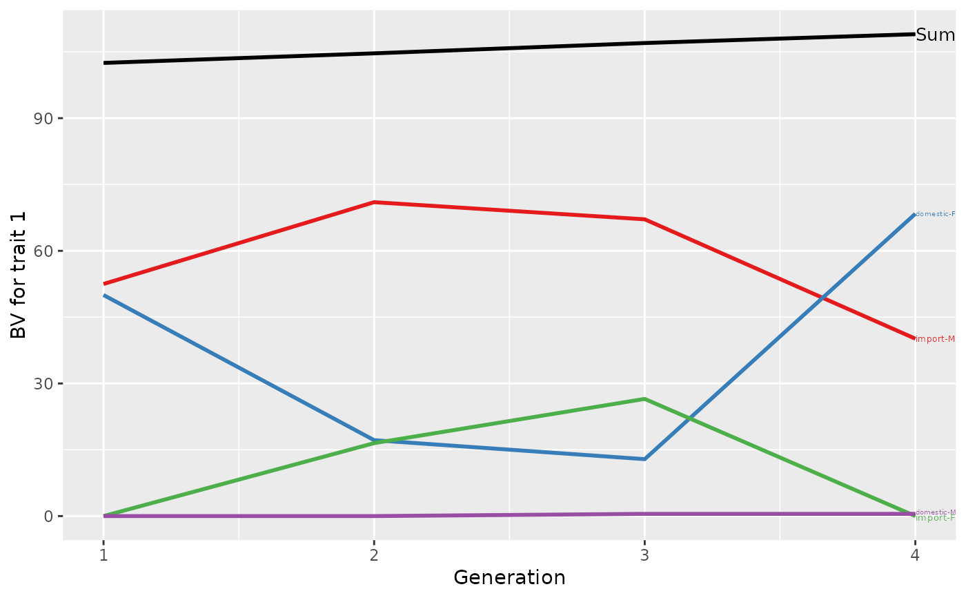
#> gen N Sum domestic-F domestic-M import-F import-M
#> 1 1 2 102.5000 50.00000 0.0 0.0 52.500
#> 2 2 3 104.6667 17.16667 0.0 16.5 71.000
#> 3 3 2 107.0000 12.87500 0.5 26.5 67.125
#> 4 4 1 109.0000 68.37500 0.5 0.0 40.125
#>
#> Trait: bv2
#>
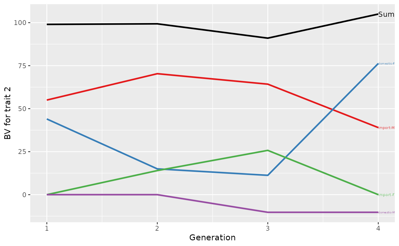
#> gen N Sum domestic-F domestic-M import-F import-M
#> 1 1 2 99.00000 44.00 0.00 0.00 55.00000
#> 2 2 3 99.33333 15.00 0.00 14.00 70.33333
#> 3 3 2 91.00000 11.25 -10.25 25.75 64.25000
#> 4 4 1 105.00000 76.25 -10.25 0.00 39.00000
#>
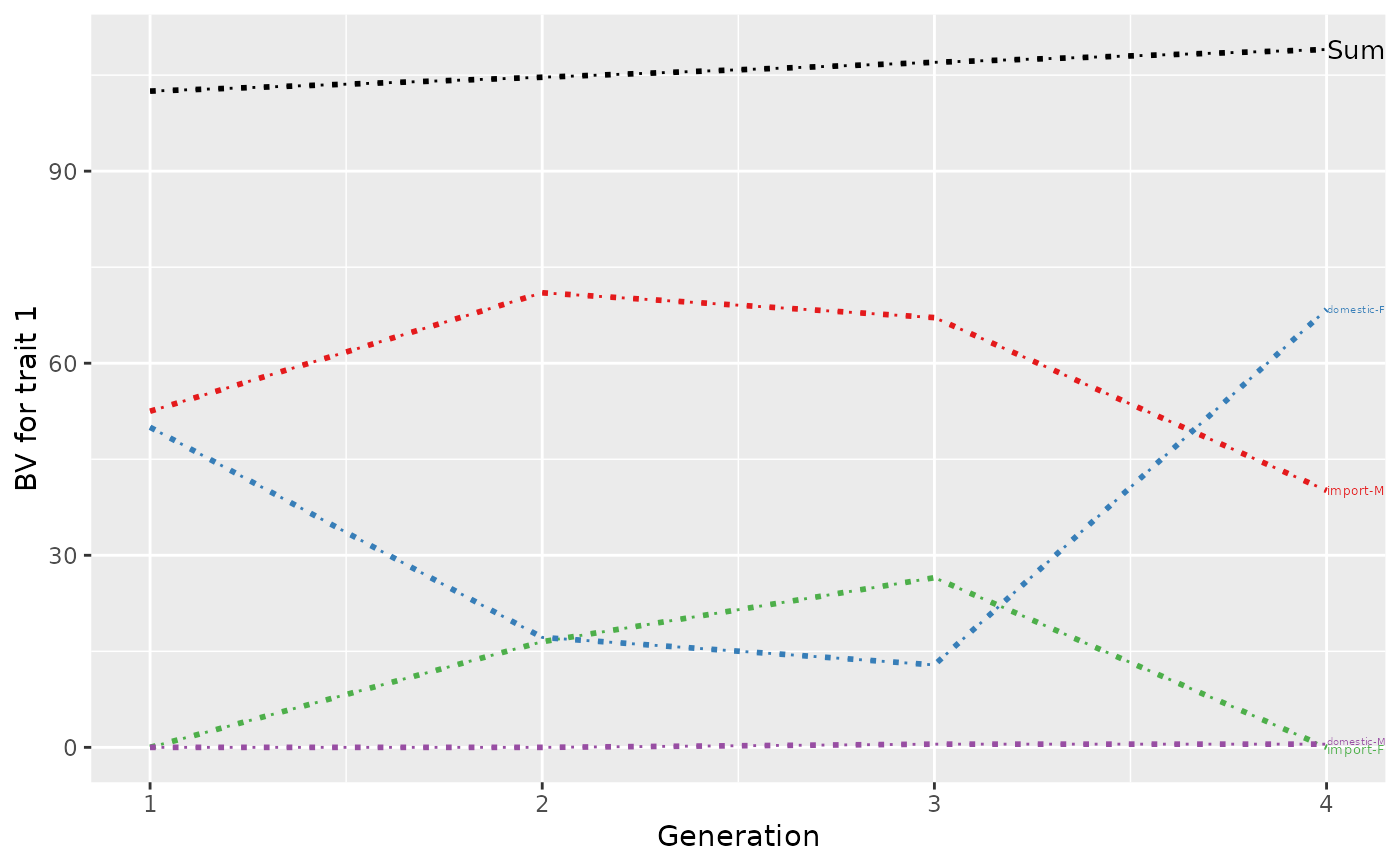
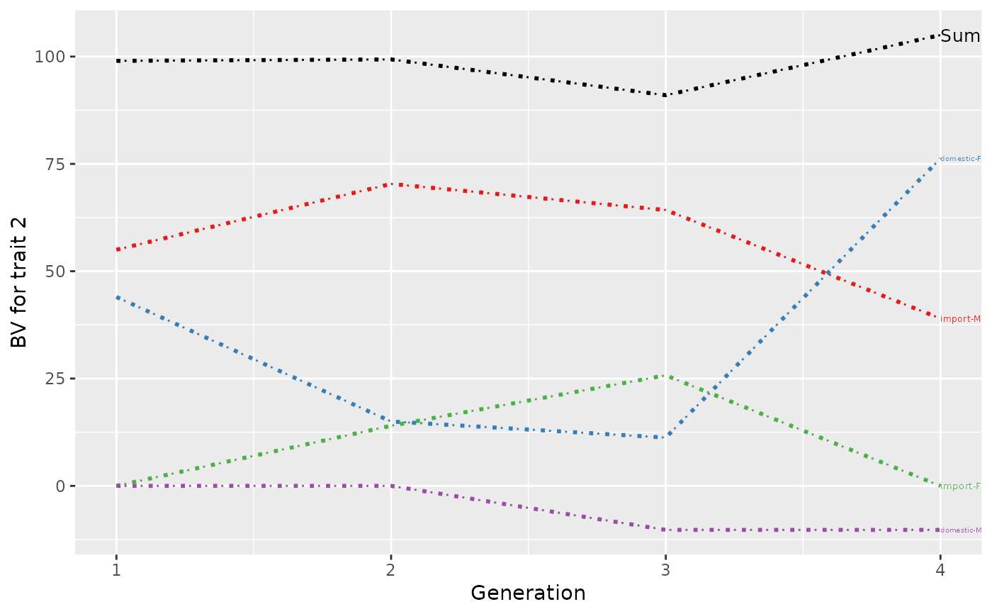
## Plot the partitions
p <- plot(ret, ylab=c("BV for trait 1", "BV for trait 2"), xlab="Generation")
print(p)
## Partition additive genetic values by country and sex
AlphaPart.ped$country.gender <- with(AlphaPart.ped, paste(country, gender, sep="-"))
(res <- AlphaPart(x=AlphaPart.ped, colPath="country.gender", colBV=c("bv1", "bv2")))
#>
#> Size:
#> - individuals: 8
#> - traits: 2 (bv1, bv2)
#> - paths: 4 (domestic-F, domestic-M, import-F, import-M)
#> - unknown (missing) values:
#> bv1 bv2
#> 0 0
#>
#>
#> Partitions of breeding values
#> - individuals: 8
#> - paths: 4 (domestic-F, domestic-M, import-F, import-M)
#> - traits: 2 (bv1, bv2)
#>
#> Trait: bv1
#>
#> IId FId MId gen country gender country.gender bv1 bv1_pa bv1_w bv1_domestic-F bv1_domestic-M bv1_import-F bv1_import-M
#> 1 A 1 domestic F domestic-F 100 104.3333 -4.3333333 100.000 0.0 0.0 0.000
#> 2 B 1 import M import-M 105 104.3333 0.6666667 0.000 0.0 0.0 105.000
#> 3 C B A 2 domestic F domestic-F 104 102.5000 1.5000000 51.500 0.0 0.0 52.500
#> 4 T B 2 import F import-F 102 52.5000 49.5000000 0.000 0.0 49.5 52.500
#> 5 D 2 import M import-M 108 104.3333 3.6666667 0.000 0.0 0.0 108.000
#> 6 E D C 3 domestic M domestic-M 107 106.0000 1.0000000 25.750 1.0 0.0 80.250
#> 7 U D 3 import F import-F 107 54.0000 53.0000000 0.000 0.0 53.0 54.000
#> 8 V E 4 domestic F domestic-F 109 53.5000 55.5000000 68.375 0.5 0.0 40.125
#>
#> Trait: bv2
#>
#> IId FId MId gen country gender country.gender bv2 bv2_pa bv2_w bv2_domestic-F bv2_domestic-M bv2_import-F bv2_import-M
#> 1 A 1 domestic F domestic-F 88 99.66667 -11.666667 88.00 0.00 0.0 0.0
#> 2 B 1 import M import-M 110 99.66667 10.333333 0.00 0.00 0.0 110.0
#> 3 C B A 2 domestic F domestic-F 100 99.00000 1.000000 45.00 0.00 0.0 55.0
#> 4 T B 2 import F import-F 97 55.00000 42.000000 0.00 0.00 42.0 55.0
#> 5 D 2 import M import-M 101 99.66667 1.333333 0.00 0.00 0.0 101.0
#> 6 E D C 3 domestic M domestic-M 80 100.50000 -20.500000 22.50 -20.50 0.0 78.0
#> 7 U D 3 import F import-F 102 50.50000 51.500000 0.00 0.00 51.5 50.5
#> 8 V E 4 domestic F domestic-F 105 40.00000 65.000000 76.25 -10.25 0.0 39.0
#>
## Summarize population by generation (=trend)
(ret <- summary(res, by="gen"))
#>
#>
#> Summary of partitions of breeding values
#> - paths: 4 (domestic-F, domestic-M, import-F, import-M)
#> - traits: 2 (bv1, bv2)
#>
#> Trait: bv1
#>
#> gen N Sum domestic-F domestic-M import-F import-M
#> 1 1 2 102.5000 50.00000 0.0 0.0 52.500
#> 2 2 3 104.6667 17.16667 0.0 16.5 71.000
#> 3 3 2 107.0000 12.87500 0.5 26.5 67.125
#> 4 4 1 109.0000 68.37500 0.5 0.0 40.125
#>
#> Trait: bv2
#>
#> gen N Sum domestic-F domestic-M import-F import-M
#> 1 1 2 99.00000 44.00 0.00 0.00 55.00000
#> 2 2 3 99.33333 15.00 0.00 14.00 70.33333
#> 3 3 2 91.00000 11.25 -10.25 25.75 64.25000
#> 4 4 1 105.00000 76.25 -10.25 0.00 39.00000
#>
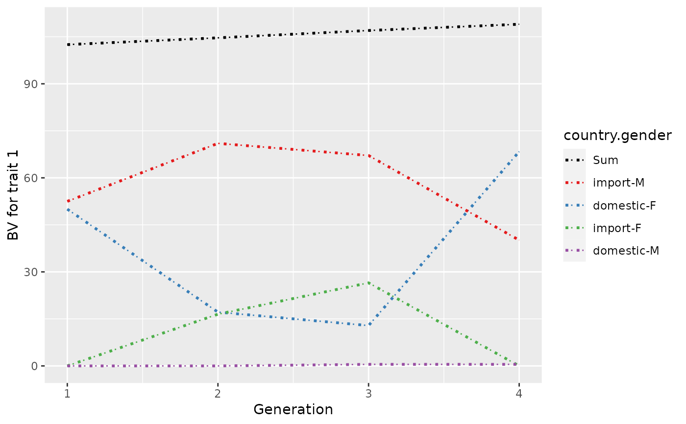
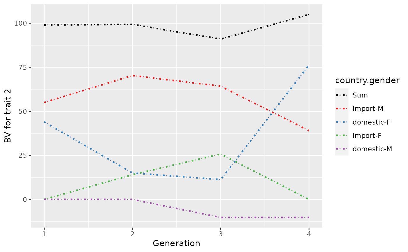
## Plot the partitions
p <- plot(ret, ylab=c("BV for trait 1", "BV for trait 2"), xlab="Generation")
print(p)
 p <- plot(ret, ylab=c("BV for trait 1", "BV for trait 2"), xlab="Generation",
lineTypeList=list("-1"=1, "-2"=2, def=3))
print(p)
p <- plot(ret, ylab=c("BV for trait 1", "BV for trait 2"), xlab="Generation",
lineTypeList=list("-1"=1, "-2"=2, def=3))
print(p)
 p <- plot(ret, ylab=c("BV for trait 1", "BV for trait 2"), xlab="Generation",
lineTypeList=list("-1"=1, "-2"=2, def=3), useGgplot2=FALSE, useDirectLabels = FALSE)
print(p)
p <- plot(ret, ylab=c("BV for trait 1", "BV for trait 2"), xlab="Generation",
lineTypeList=list("-1"=1, "-2"=2, def=3), useGgplot2=FALSE, useDirectLabels = FALSE)
print(p)
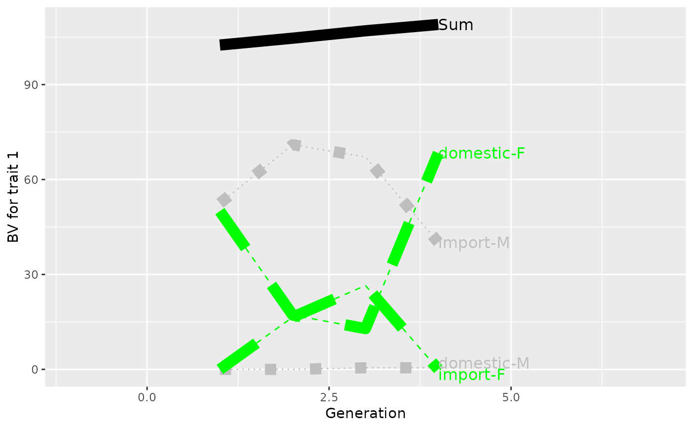
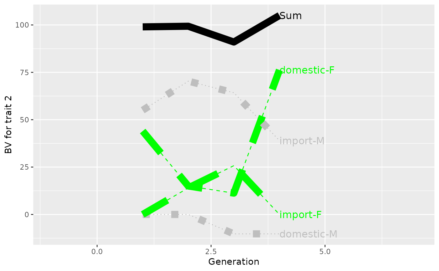
 ## Plot control (color and type of lines + limits)
p <- plot(ret, ylab=c("BV for trait 1", "BV for trait 2"), xlab="Generation",
useGgplot2=TRUE, color=c("green", "gray"), lineType=c(2, 3),
sortValue=FALSE, lineSize=4,
xlim=c(-1, 7))
print(p)
## Plot control (color and type of lines + limits)
p <- plot(ret, ylab=c("BV for trait 1", "BV for trait 2"), xlab="Generation",
useGgplot2=TRUE, color=c("green", "gray"), lineType=c(2, 3),
sortValue=FALSE, lineSize=4,
xlim=c(-1, 7))
print(p)
 # }
# }