Print method for the output of AlphaPart function.
print.AlphaPart.RdPartitioning of breeding values if often performed on
quite large datasets, which quickly fills in the whole
screen. Print method therefore prints out paths, number of
individuals and the first and the last few lines for each trait to
quickly see what kind of data is in x.
Usage
# S3 method for class 'AlphaPart'
print(x, n, ...)Examples
## Small pedigree with additive genetic (=breeding) values
ped <- data.frame( id=c( 1, 2, 3, 4, 5, 6),
fid=c( 0, 0, 2, 0, 4, 0),
mid=c( 0, 0, 1, 0, 3, 3),
loc=c("A", "B", "A", "B", "A", "A"),
gen=c( 1, 1, 2, 2, 3, 3),
trt1=c(100, 120, 115, 130, 125, 125),
trt2=c(100, 110, 105, 100, 85, 110))
## Partition additive genetic values
tmp <- AlphaPart(x=ped, colBV=c("trt1", "trt2"))
#>
#> Size:
#> - individuals: 6
#> - traits: 2 (trt1, trt2)
#> - paths: 2 (A, B)
#> - unknown (missing) values:
#> trt1 trt2
#> 0 0
print(tmp)
#>
#>
#> Partitions of breeding values
#> - individuals: 6
#> - paths: 2 (A, B)
#> - traits: 2 (trt1, trt2)
#>
#> Trait: trt1
#>
#> id fid mid loc gen trt1 trt1_pa trt1_w trt1_A trt1_B
#> 1 1 0 0 A 1 100 116.6667 -16.666667 100 0
#> 2 2 0 0 B 1 120 116.6667 3.333333 0 120
#> 3 3 2 1 A 2 115 110.0000 5.000000 55 60
#> 4 4 0 0 B 2 130 116.6667 13.333333 0 130
#> 5 5 4 3 A 3 125 122.5000 2.500000 30 95
#> 6 6 0 3 A 3 125 57.5000 67.500000 95 30
#>
#> Trait: trt2
#>
#> id fid mid loc gen trt2 trt2_pa trt2_w trt2_A trt2_B
#> 1 1 0 0 A 1 100 103.3333 -3.333333 100.0 0.0
#> 2 2 0 0 B 1 110 103.3333 6.666667 0.0 110.0
#> 3 3 2 1 A 2 105 105.0000 0.000000 50.0 55.0
#> 4 4 0 0 B 2 100 103.3333 -3.333333 0.0 100.0
#> 5 5 4 3 A 3 85 102.5000 -17.500000 7.5 77.5
#> 6 6 0 3 A 3 110 52.5000 57.500000 82.5 27.5
#>
## Summarize by generation (genetic mean)
summary(tmp, by="gen")
#>
#>
#> Summary of partitions of breeding values
#> - paths: 2 (A, B)
#> - traits: 2 (trt1, trt2)
#>
#> Trait: trt1
#>
#> gen N Sum A B
#> 1 1 2 110.0 50.0 60.0
#> 2 2 2 122.5 27.5 95.0
#> 3 3 2 125.0 62.5 62.5
#>
#> Trait: trt2
#>
#> gen N Sum A B
#> 1 1 2 105.0 50 55.0
#> 2 2 2 102.5 25 77.5
#> 3 3 2 97.5 45 52.5
#>
## Summarize by generation (genetic variance)
summary(tmp, by="gen", FUN = var)
#>
#>
#> Summary of partitions of breeding values
#> - paths: 2 (A, B, Sum.Cov)
#> - traits: 2 (trt1, trt2)
#>
#> Trait: trt1
#>
#> gen N Sum A B Sum.Cov
#> 1 1 2 200.0 5000.0 7200.0 -12000
#> 2 2 2 112.5 1512.5 2450.0 -3850
#> 3 3 2 0.0 2112.5 2112.5 -4225
#>
#> Trait: trt2
#>
#> gen N Sum A B Sum.Cov
#> 1 1 2 50.0 5000.0 6050.0 -11000
#> 2 2 2 12.5 1250.0 1012.5 -2250
#> 3 3 2 312.5 2812.5 1250.0 -3750
#>
# \donttest{
## There are also two demos
demo(topic="AlphaPart_deterministic", package="AlphaPart",
ask=interactive())
#>
#>
#> demo(AlphaPart_deterministic)
#> ---- ~~~~~~~~~~~~~~~~~~~~~~~
#>
#> > ### partAGV_deterministic.R
#> > ###-----------------------------------------------------------------------------
#> > ### $Id$
#> > ###-----------------------------------------------------------------------------
#> >
#> > ### DESCRIPTION OF A DEMONSTRATION
#> > ###-----------------------------------------------------------------------------
#> >
#> > ## A demonstration with a simple example to see in action the partitioning of
#> > ## additive genetic values by paths (Garcia-Cortes et al., 2008; Animal)
#> > ##
#> > ## DETERMINISTIC SIMULATION (sort of)
#> > ##
#> > ## We have two locations (1 and 2). The first location has individualss with higher
#> > ## additive genetic value. Males from the first location are imported males to the
#> > ## second location from generation 2/3. This clearly leads to genetic gain in the
#> > ## second location. However, the second location can also perform their own selection
#> > ## so the question is how much genetic gain is due to the import of genes from the
#> > ## first location and due to their own selection.
#> > ##
#> > ## Above scenario will be tested with a simple example of a pedigree bellow. Two
#> > ## scenarios will be evaluated: without or with own selection in the second location.
#> > ## Selection will always be present in the first location.
#> > ##
#> > ## Additive genetic values are provided, i.e., no inference is being done!
#> > ##
#> > ## The idea of this example is not to do extensive simulations, but just to have
#> > ## a simple example to see how the partitioning of additive genetic values works.
#> >
#> > ### SETUP
#> > ###-----------------------------------------------------------------------------
#> >
#> > options(width=200)
#>
#> > ### EXAMPLE PEDIGREE & SETUP OF MENDELIAN SAMPLING - "DETERMINISTIC"
#> > ###-----------------------------------------------------------------------------
#> >
#> > ## Generation 0
#> > id0 <- c("01", "02", "03", "04")
#>
#> > fid0 <- mid0 <- rep(NA, times=length(id0))
#>
#> > h0 <- rep(c(1, 2), each=2)
#>
#> > g0 <- rep(0, times=length(id0))
#>
#> > w10 <- c( 2, 2, 0, 0)
#>
#> > w20 <- c( 2, 2, 0, 0)
#>
#> > ## Generation 1
#> > id1 <- c("11", "12", "13", "14")
#>
#> > fid1 <- c("01", "01", "03", "03")
#>
#> > mid1 <- c("02", "02", "04", "04")
#>
#> > h1 <- h0
#>
#> > g1 <- rep(1, times=length(id1))
#>
#> > w11 <- c( 0.6, 0.2, -0.6, 0.2)
#>
#> > w21 <- c( 0.6, 0.2, 0.6, 0.2)
#>
#> > ## Generation 2
#> > id2 <- c("21", "22", "23", "24")
#>
#> > fid2 <- c("12", "12", "12", "12")
#>
#> > mid2 <- c("11", "11", "13", "14")
#>
#> > h2 <- h0
#>
#> > g2 <- rep(2, times=length(id2))
#>
#> > w12 <- c( 0.6, 0.3, -0.2, 0.2)
#>
#> > w22 <- c( 0.6, 0.3, 0.2, 0.2)
#>
#> > ## Generation 3
#> > id3 <- c("31", "32", "33", "34")
#>
#> > fid3 <- c("22", "22", "22", "22")
#>
#> > mid3 <- c("21", "21", "23", "24")
#>
#> > h3 <- h0
#>
#> > g3 <- rep(3, times=length(id3))
#>
#> > w13 <- c( 0.7, 0.1, -0.3, 0.3)
#>
#> > w23 <- c( 0.7, 0.1, 0.3, 0.3)
#>
#> > ## Generation 4
#> > id4 <- c("41", "42", "43", "44")
#>
#> > fid4 <- c("32", "32", "32", "32")
#>
#> > mid4 <- c("31", "31", "33", "34")
#>
#> > h4 <- h0
#>
#> > g4 <- rep(4, times=length(id4))
#>
#> > w14 <- c( 0.8, 0.8, -0.1, 0.3)
#>
#> > w24 <- c( 0.8, 0.8, 0.1, 0.3)
#>
#> > ## Generation 5
#> > id5 <- c("51", "52", "53", "54")
#>
#> > fid5 <- c("42", "42", "42", "42")
#>
#> > mid5 <- c("41", "41", "43", "44")
#>
#> > h5 <- h0
#>
#> > g5 <- rep(5, times=length(id4))
#>
#> > w15 <- c( 0.8, 1.0, -0.2, 0.3)
#>
#> > w25 <- c( 0.8, 1.0, 0.2, 0.3)
#>
#> > ped <- data.frame( id=c( id0, id1, id2, id3, id4, id5),
#> + fid=c(fid0, fid1, fid2, fid3, fid4, fid5),
#> + mid=c(mid0, mid1, mid2, mid3, mid4, mid5),
#> + loc=c( h0, h1, h2, h3, h4, h5),
#> + gen=c( g0, g1, g2, g3, g4, g5),
#> + w1=c( w10, w11, w12, w13, w14, w15),
#> + w2=c( w20, w21, w22, w23, w24, w25))
#>
#> > ped$sex <- 2
#>
#> > ped[ped$id %in% ped$fid, "sex"] <- 1
#>
#> > ped$loc.gen <- with(ped, paste(loc, gen, sep="-"))
#>
#> > ### SIMULATE ADDITIVE GENETIC VALUES - SUM PARENT AVERAGE AND MENDELIAN SAMPLING
#> > ###-----------------------------------------------------------------------------
#> >
#> > ## Additive genetic mean in founders by location
#> > mu1 <- 2
#>
#> > mu2 <- 0
#>
#> > ## Additive genetic variance in population
#> > sigma2 <- 1
#>
#> > sigma <- sqrt(sigma2)
#>
#> > ## Threshold value for Mendelian sampling for selection - only values above this
#> > ## will be accepted in simulation
#> > t <- 0
#>
#> > ped$agv1 <- ped$pa1 <- NA ## Scenario (trait) 1: No selection in the second location
#>
#> > ped$agv2 <- ped$pa2 <- NA ## Scenario (trait) 2: Selection in the second location
#>
#> > ## Generation 0 - founders (no parent average here - so setting it to zero)
#> > ped[ped$gen == 0, c("pa1", "pa2")] <- 0
#>
#> > ped[ped$gen == 0, c("agv1", "agv2")] <- ped[ped$gen == 0, c("w1", "w2")]
#>
#> > ## Generation 1+ - non-founders (parent average + Mendelian sampling)
#> > for(i in (length(g0)+1):nrow(ped)) {
#> + ped[i, "pa1"] <- 0.5 * (ped[ped$id %in% ped[i, "fid"], "agv1"] +
#> + ped[ped$id %in% ped[i, "mid"], "agv1"])
#> + ped[i, "pa2"] <- 0.5 * (ped[ped$id %in% ped[i, "fid"], "agv2"] +
#> + ped[ped$id %in% ped[i, "mid"], "agv2"])
#> + ped[i, c("agv1", "agv2")] <- ped[i, c("pa1", "pa2")] + ped[i, c("w1", "w2")]
#> + }
#>
#> > ### PLOT INDIVIDUAL ADDITIVE GENETIC VALUES
#> > ###-----------------------------------------------------------------------------
#> >
#> > par(mfrow=c(2, 1), bty="l", pty="m", mar=c(2, 2, 1, 1) + .1, mgp=c(0.7, 0.2, 0))
#>
#> > tmp <- ped$gen + c(-1.5, -0.5, 0.5, 1.5) * 0.1
#>
#> > with(ped, plot(agv1 ~ tmp, pch=c(19, 21)[ped$loc], ylab="Additive genetic value",
#> + xlab="Generation", main="Selection in location 1", axes=FALSE,
#> + ylim=range(c(agv1, agv2))))
#>
#> > axis(1, labels=FALSE, tick=FALSE); axis(2, labels=FALSE, tick=FALSE); box()
#>
#> > legend(x="topleft", legend=c(1, 2), title="Location", pch=c(19, 21), bty="n")
#>
#> > with(ped, plot(agv2 ~ tmp, pch=c(19, 21)[ped$loc], ylab="Additive genetic value",
#> + xlab="Generation", main="Selection in locations 1 and 2", axes=FALSE,
#> + ylim=range(c(agv1, agv2))))
 #>
#> > axis(1, labels=FALSE, tick=FALSE); axis(2, labels=FALSE, tick=FALSE); box()
#>
#> > legend(x="topleft", legend=c(1, 2), title="Location", pch=c(19, 21), bty="n")
#>
#> > ### PARTITION ADDITIVE GENETIC VALUES BY ...
#> > ###-----------------------------------------------------------------------------
#> >
#> > ## Compute partitions by location
#> > (res <- AlphaPart(x=ped, colPath="loc", colBV=c("agv1", "agv2")))
#>
#> Size:
#> - individuals: 24
#> - traits: 2 (agv1, agv2)
#> - paths: 2 (1, 2)
#> - unknown (missing) values:
#> agv1 agv2
#> 0 0
#>
#>
#> Partitions of breeding values
#> - individuals: 24
#> - paths: 2 (1, 2)
#> - traits: 2 (agv1, agv2)
#>
#> Trait: agv1
#>
#> id fid mid loc gen w1 w2 sex loc.gen pa1 pa2 agv1 agv1_pa agv1_w agv1_1 agv1_2
#> 1 01 <NA> <NA> 1 0 2.0 2.0 1 1-0 0 0 2.0 0 2.0 2.0 0
#> 2 02 <NA> <NA> 1 0 2.0 2.0 2 1-0 0 0 2.0 0 2.0 2.0 0
#> 3 03 <NA> <NA> 2 0 0.0 0.0 1 2-0 0 0 0.0 0 0.0 0.0 0
#> 4 04 <NA> <NA> 2 0 0.0 0.0 2 2-0 0 0 0.0 0 0.0 0.0 0
#> 5 11 01 02 1 1 0.6 0.6 2 1-1 2 2 2.6 2 0.6 2.6 0
#> 6 12 01 02 1 1 0.2 0.2 1 1-1 2 2 2.2 2 0.2 2.2 0
#> ...
#> id fid mid loc gen w1 w2 sex loc.gen pa1 pa2 agv1 agv1_pa agv1_w agv1_1 agv1_2
#> 19 43 32 33 2 4 -0.1 0.1 2 2-4 2.15 2.700 2.05 2.15 -0.1 2.4250 -0.3750
#> 20 44 32 34 2 4 0.3 0.3 2 2-4 2.65 2.650 2.95 2.65 0.3 2.4250 0.5250
#> 21 51 42 41 1 5 0.8 0.8 2 1-5 4.05 4.050 4.85 4.05 0.8 4.8500 0.0000
#> 22 52 42 41 1 5 1.0 1.0 2 1-5 4.05 4.050 5.05 4.05 1.0 5.0500 0.0000
#> 23 53 42 43 2 5 -0.2 0.2 2 2-5 3.05 3.425 2.85 3.05 -0.2 3.2375 -0.3875
#> 24 54 42 44 2 5 0.3 0.3 2 2-5 3.50 3.500 3.80 3.50 0.3 3.2375 0.5625
#>
#> Trait: agv2
#>
#> id fid mid loc gen w1 w2 sex loc.gen pa1 pa2 agv2 agv2_pa agv2_w agv2_1 agv2_2
#> 1 01 <NA> <NA> 1 0 2.0 2.0 1 1-0 0 0 2.0 0 2.0 2.0 0
#> 2 02 <NA> <NA> 1 0 2.0 2.0 2 1-0 0 0 2.0 0 2.0 2.0 0
#> 3 03 <NA> <NA> 2 0 0.0 0.0 1 2-0 0 0 0.0 0 0.0 0.0 0
#> 4 04 <NA> <NA> 2 0 0.0 0.0 2 2-0 0 0 0.0 0 0.0 0.0 0
#> 5 11 01 02 1 1 0.6 0.6 2 1-1 2 2 2.6 2 0.6 2.6 0
#> 6 12 01 02 1 1 0.2 0.2 1 1-1 2 2 2.2 2 0.2 2.2 0
#> ...
#> id fid mid loc gen w1 w2 sex loc.gen pa1 pa2 agv2 agv2_pa agv2_w agv2_1 agv2_2
#> 19 43 32 33 2 4 -0.1 0.1 2 2-4 2.15 2.700 2.800 2.700 0.1 2.4250 0.3750
#> 20 44 32 34 2 4 0.3 0.3 2 2-4 2.65 2.650 2.950 2.650 0.3 2.4250 0.5250
#> 21 51 42 41 1 5 0.8 0.8 2 1-5 4.05 4.050 4.850 4.050 0.8 4.8500 0.0000
#> 22 52 42 41 1 5 1.0 1.0 2 1-5 4.05 4.050 5.050 4.050 1.0 5.0500 0.0000
#> 23 53 42 43 2 5 -0.2 0.2 2 2-5 3.05 3.425 3.625 3.425 0.2 3.2375 0.3875
#> 24 54 42 44 2 5 0.3 0.3 2 2-5 3.50 3.500 3.800 3.500 0.3 3.2375 0.5625
#>
#>
#> > ## Summarize whole population
#> > (ret <- summary(res))
#>
#>
#> Summary of partitions of breeding values
#> - paths: 2 (1, 2)
#> - traits: 2 (agv1, agv2)
#>
#> Trait: agv1
#>
#> N <NA> Sum 1 2
#> 1 1 24 2.33125 2.346875 -0.015625
#>
#> Trait: agv2
#>
#> N <NA> Sum 1 2
#> 1 1 24 2.532292 2.346875 0.1854167
#>
#>
#> > ## Summarize and plot by generation (=trend)
#> > (ret <- summary(res, by="gen"))
#>
#>
#> Summary of partitions of breeding values
#> - paths: 2 (1, 2)
#> - traits: 2 (agv1, agv2)
#>
#> Trait: agv1
#>
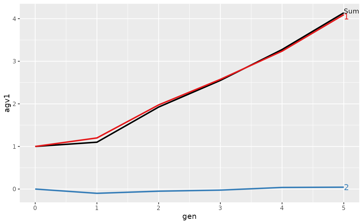
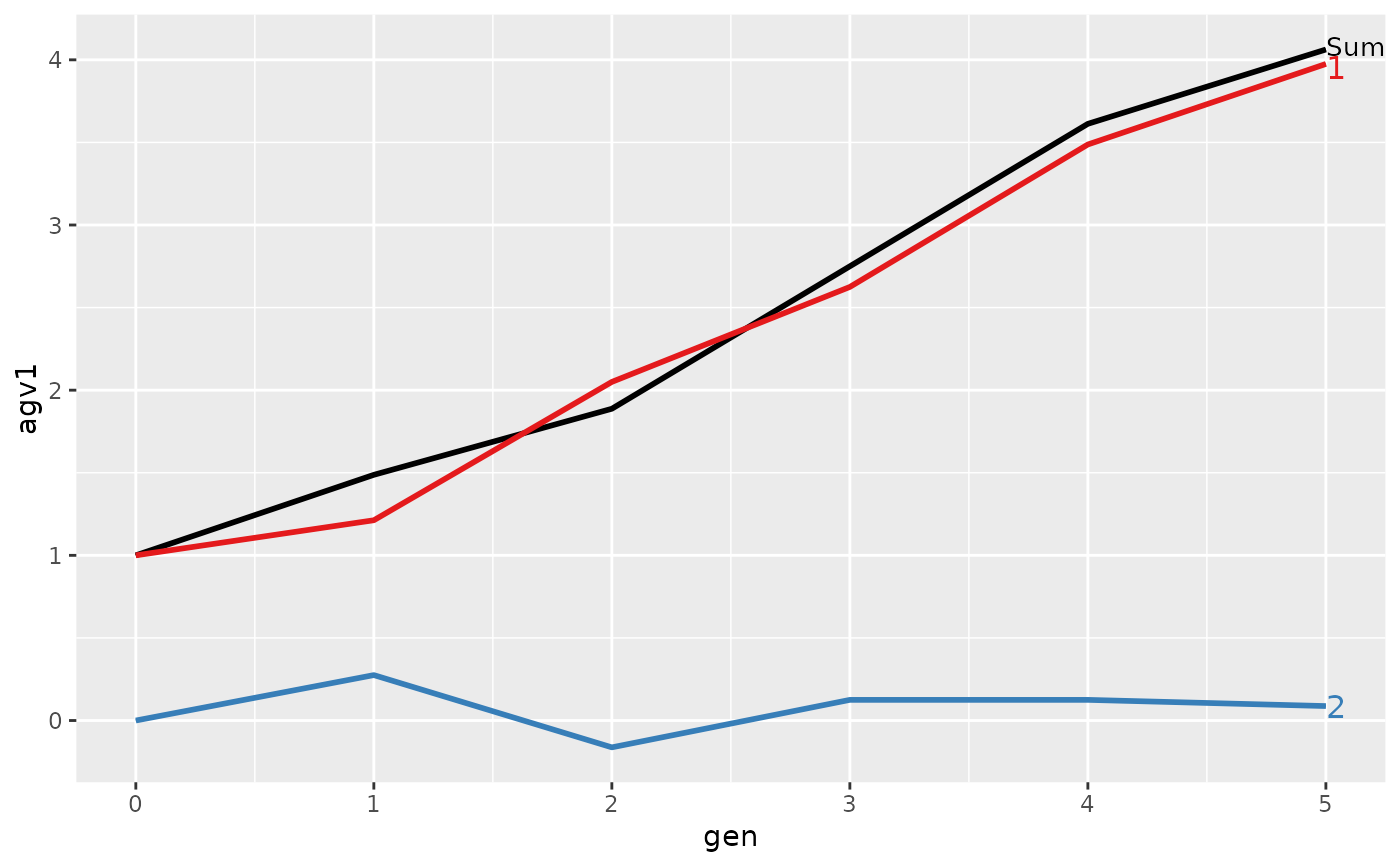
#> gen N Sum 1 2
#> 1 0 4 1.0000 1.00000 0.00000
#> 2 1 4 1.1000 1.20000 -0.10000
#> 3 2 4 1.9250 1.97500 -0.05000
#> 4 3 4 2.5500 2.57500 -0.02500
#> 5 4 4 3.2750 3.23750 0.03750
#> 6 5 4 4.1375 4.09375 0.04375
#>
#> Trait: agv2
#>
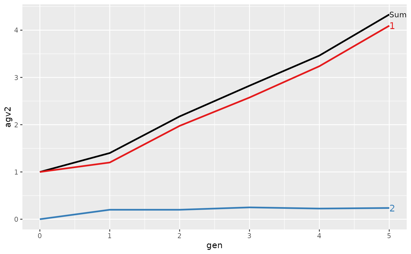
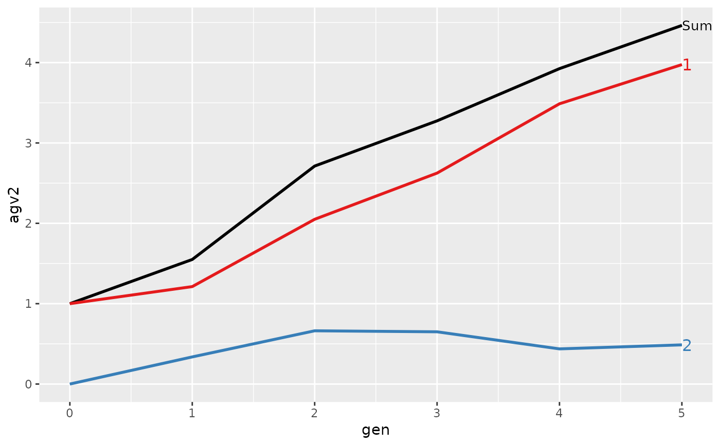
#> gen N Sum 1 2
#> 1 0 4 1.00000 1.00000 0.0000
#> 2 1 4 1.40000 1.20000 0.2000
#> 3 2 4 2.17500 1.97500 0.2000
#> 4 3 4 2.82500 2.57500 0.2500
#> 5 4 4 3.46250 3.23750 0.2250
#> 6 5 4 4.33125 4.09375 0.2375
#>
#>
#> > plot(ret)
#>
#> > axis(1, labels=FALSE, tick=FALSE); axis(2, labels=FALSE, tick=FALSE); box()
#>
#> > legend(x="topleft", legend=c(1, 2), title="Location", pch=c(19, 21), bty="n")
#>
#> > ### PARTITION ADDITIVE GENETIC VALUES BY ...
#> > ###-----------------------------------------------------------------------------
#> >
#> > ## Compute partitions by location
#> > (res <- AlphaPart(x=ped, colPath="loc", colBV=c("agv1", "agv2")))
#>
#> Size:
#> - individuals: 24
#> - traits: 2 (agv1, agv2)
#> - paths: 2 (1, 2)
#> - unknown (missing) values:
#> agv1 agv2
#> 0 0
#>
#>
#> Partitions of breeding values
#> - individuals: 24
#> - paths: 2 (1, 2)
#> - traits: 2 (agv1, agv2)
#>
#> Trait: agv1
#>
#> id fid mid loc gen w1 w2 sex loc.gen pa1 pa2 agv1 agv1_pa agv1_w agv1_1 agv1_2
#> 1 01 <NA> <NA> 1 0 2.0 2.0 1 1-0 0 0 2.0 0 2.0 2.0 0
#> 2 02 <NA> <NA> 1 0 2.0 2.0 2 1-0 0 0 2.0 0 2.0 2.0 0
#> 3 03 <NA> <NA> 2 0 0.0 0.0 1 2-0 0 0 0.0 0 0.0 0.0 0
#> 4 04 <NA> <NA> 2 0 0.0 0.0 2 2-0 0 0 0.0 0 0.0 0.0 0
#> 5 11 01 02 1 1 0.6 0.6 2 1-1 2 2 2.6 2 0.6 2.6 0
#> 6 12 01 02 1 1 0.2 0.2 1 1-1 2 2 2.2 2 0.2 2.2 0
#> ...
#> id fid mid loc gen w1 w2 sex loc.gen pa1 pa2 agv1 agv1_pa agv1_w agv1_1 agv1_2
#> 19 43 32 33 2 4 -0.1 0.1 2 2-4 2.15 2.700 2.05 2.15 -0.1 2.4250 -0.3750
#> 20 44 32 34 2 4 0.3 0.3 2 2-4 2.65 2.650 2.95 2.65 0.3 2.4250 0.5250
#> 21 51 42 41 1 5 0.8 0.8 2 1-5 4.05 4.050 4.85 4.05 0.8 4.8500 0.0000
#> 22 52 42 41 1 5 1.0 1.0 2 1-5 4.05 4.050 5.05 4.05 1.0 5.0500 0.0000
#> 23 53 42 43 2 5 -0.2 0.2 2 2-5 3.05 3.425 2.85 3.05 -0.2 3.2375 -0.3875
#> 24 54 42 44 2 5 0.3 0.3 2 2-5 3.50 3.500 3.80 3.50 0.3 3.2375 0.5625
#>
#> Trait: agv2
#>
#> id fid mid loc gen w1 w2 sex loc.gen pa1 pa2 agv2 agv2_pa agv2_w agv2_1 agv2_2
#> 1 01 <NA> <NA> 1 0 2.0 2.0 1 1-0 0 0 2.0 0 2.0 2.0 0
#> 2 02 <NA> <NA> 1 0 2.0 2.0 2 1-0 0 0 2.0 0 2.0 2.0 0
#> 3 03 <NA> <NA> 2 0 0.0 0.0 1 2-0 0 0 0.0 0 0.0 0.0 0
#> 4 04 <NA> <NA> 2 0 0.0 0.0 2 2-0 0 0 0.0 0 0.0 0.0 0
#> 5 11 01 02 1 1 0.6 0.6 2 1-1 2 2 2.6 2 0.6 2.6 0
#> 6 12 01 02 1 1 0.2 0.2 1 1-1 2 2 2.2 2 0.2 2.2 0
#> ...
#> id fid mid loc gen w1 w2 sex loc.gen pa1 pa2 agv2 agv2_pa agv2_w agv2_1 agv2_2
#> 19 43 32 33 2 4 -0.1 0.1 2 2-4 2.15 2.700 2.800 2.700 0.1 2.4250 0.3750
#> 20 44 32 34 2 4 0.3 0.3 2 2-4 2.65 2.650 2.950 2.650 0.3 2.4250 0.5250
#> 21 51 42 41 1 5 0.8 0.8 2 1-5 4.05 4.050 4.850 4.050 0.8 4.8500 0.0000
#> 22 52 42 41 1 5 1.0 1.0 2 1-5 4.05 4.050 5.050 4.050 1.0 5.0500 0.0000
#> 23 53 42 43 2 5 -0.2 0.2 2 2-5 3.05 3.425 3.625 3.425 0.2 3.2375 0.3875
#> 24 54 42 44 2 5 0.3 0.3 2 2-5 3.50 3.500 3.800 3.500 0.3 3.2375 0.5625
#>
#>
#> > ## Summarize whole population
#> > (ret <- summary(res))
#>
#>
#> Summary of partitions of breeding values
#> - paths: 2 (1, 2)
#> - traits: 2 (agv1, agv2)
#>
#> Trait: agv1
#>
#> N <NA> Sum 1 2
#> 1 1 24 2.33125 2.346875 -0.015625
#>
#> Trait: agv2
#>
#> N <NA> Sum 1 2
#> 1 1 24 2.532292 2.346875 0.1854167
#>
#>
#> > ## Summarize and plot by generation (=trend)
#> > (ret <- summary(res, by="gen"))
#>
#>
#> Summary of partitions of breeding values
#> - paths: 2 (1, 2)
#> - traits: 2 (agv1, agv2)
#>
#> Trait: agv1
#>
#> gen N Sum 1 2
#> 1 0 4 1.0000 1.00000 0.00000
#> 2 1 4 1.1000 1.20000 -0.10000
#> 3 2 4 1.9250 1.97500 -0.05000
#> 4 3 4 2.5500 2.57500 -0.02500
#> 5 4 4 3.2750 3.23750 0.03750
#> 6 5 4 4.1375 4.09375 0.04375
#>
#> Trait: agv2
#>
#> gen N Sum 1 2
#> 1 0 4 1.00000 1.00000 0.0000
#> 2 1 4 1.40000 1.20000 0.2000
#> 3 2 4 2.17500 1.97500 0.2000
#> 4 3 4 2.82500 2.57500 0.2500
#> 5 4 4 3.46250 3.23750 0.2250
#> 6 5 4 4.33125 4.09375 0.2375
#>
#>
#> > plot(ret)
 #>
#> > ## Summarize and plot location specific trends
#> > (ret <- summary(res, by="loc.gen"))
#>
#>
#> Summary of partitions of breeding values
#> - paths: 2 (1, 2)
#> - traits: 2 (agv1, agv2)
#>
#> Trait: agv1
#>
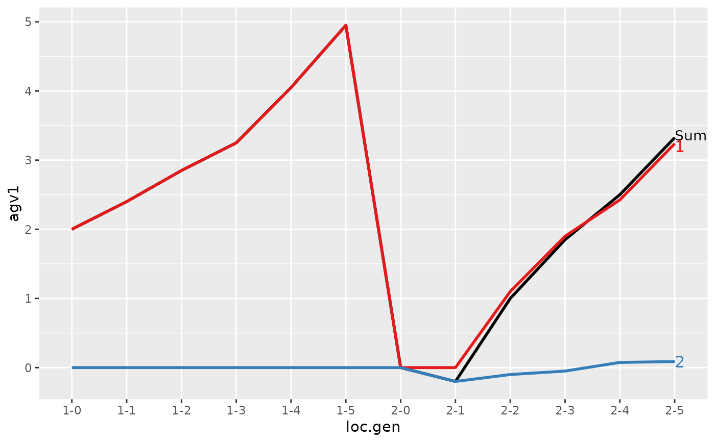
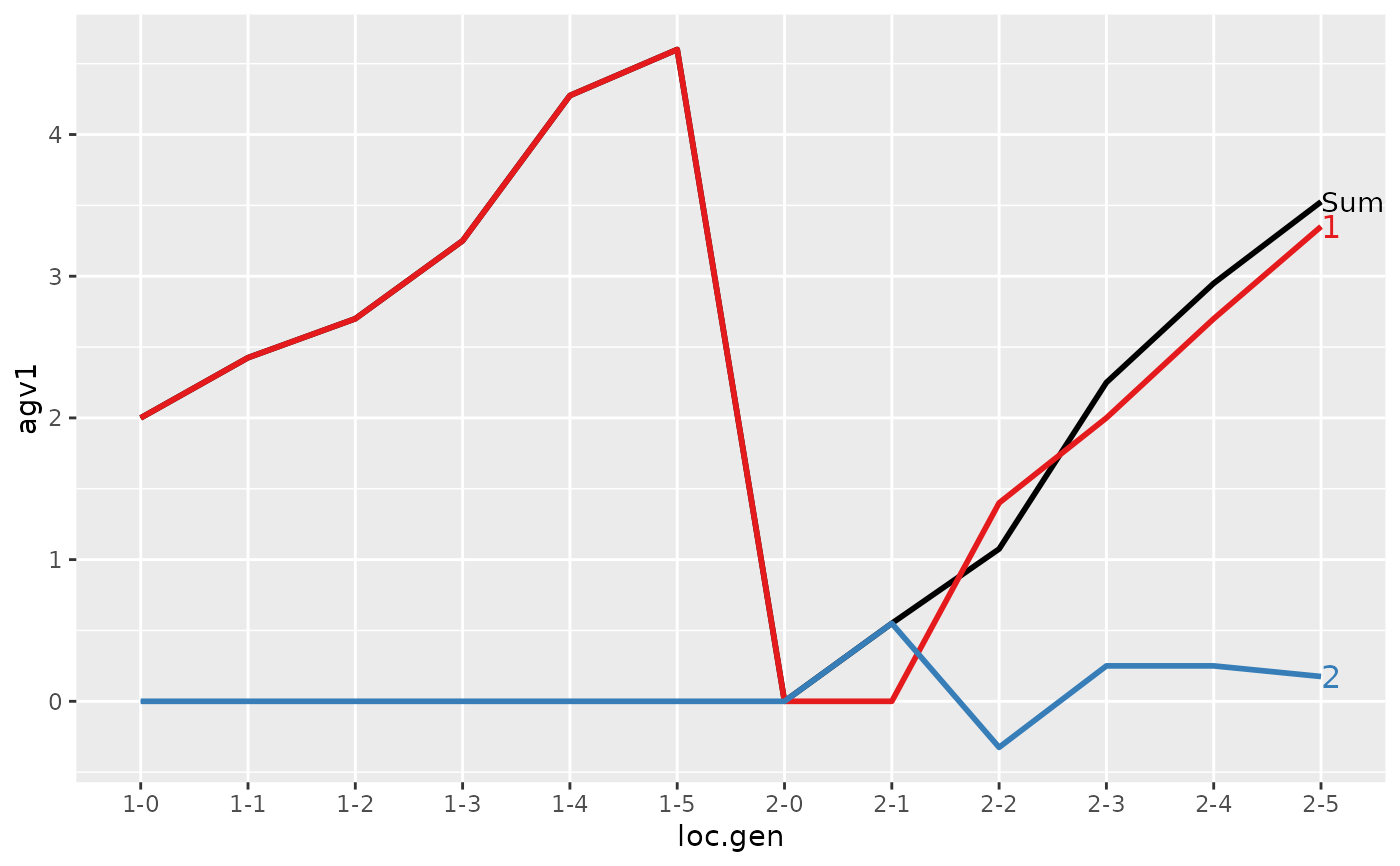
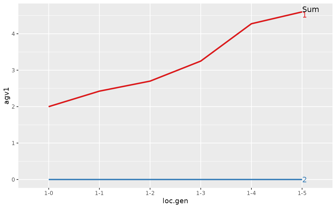
#> loc.gen N Sum 1 2
#> 1 1-0 2 2.000 2.0000 0.0000
#> 2 1-1 2 2.400 2.4000 0.0000
#> 3 1-2 2 2.850 2.8500 0.0000
#> 4 1-3 2 3.250 3.2500 0.0000
#> 5 1-4 2 4.050 4.0500 0.0000
#> 6 1-5 2 4.950 4.9500 0.0000
#> 7 2-0 2 0.000 0.0000 0.0000
#> 8 2-1 2 -0.200 0.0000 -0.2000
#> 9 2-2 2 1.000 1.1000 -0.1000
#> 10 2-3 2 1.850 1.9000 -0.0500
#> 11 2-4 2 2.500 2.4250 0.0750
#> 12 2-5 2 3.325 3.2375 0.0875
#>
#> Trait: agv2
#>
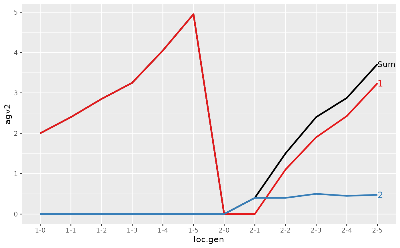
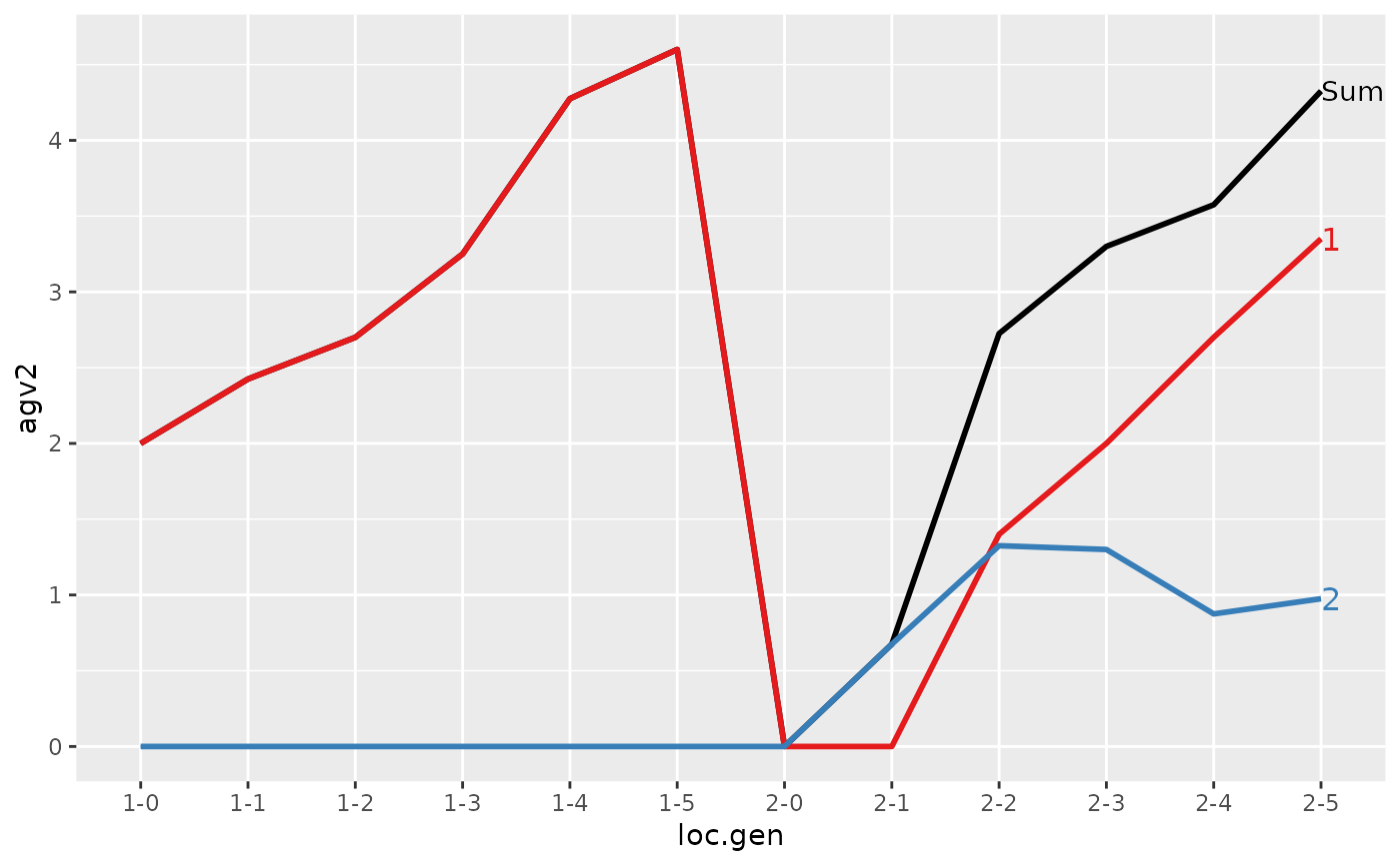
#> loc.gen N Sum 1 2
#> 1 1-0 2 2.0000 2.0000 0.000
#> 2 1-1 2 2.4000 2.4000 0.000
#> 3 1-2 2 2.8500 2.8500 0.000
#> 4 1-3 2 3.2500 3.2500 0.000
#> 5 1-4 2 4.0500 4.0500 0.000
#> 6 1-5 2 4.9500 4.9500 0.000
#> 7 2-0 2 0.0000 0.0000 0.000
#> 8 2-1 2 0.4000 0.0000 0.400
#> 9 2-2 2 1.5000 1.1000 0.400
#> 10 2-3 2 2.4000 1.9000 0.500
#> 11 2-4 2 2.8750 2.4250 0.450
#> 12 2-5 2 3.7125 3.2375 0.475
#>
#>
#> > plot(ret)
#>
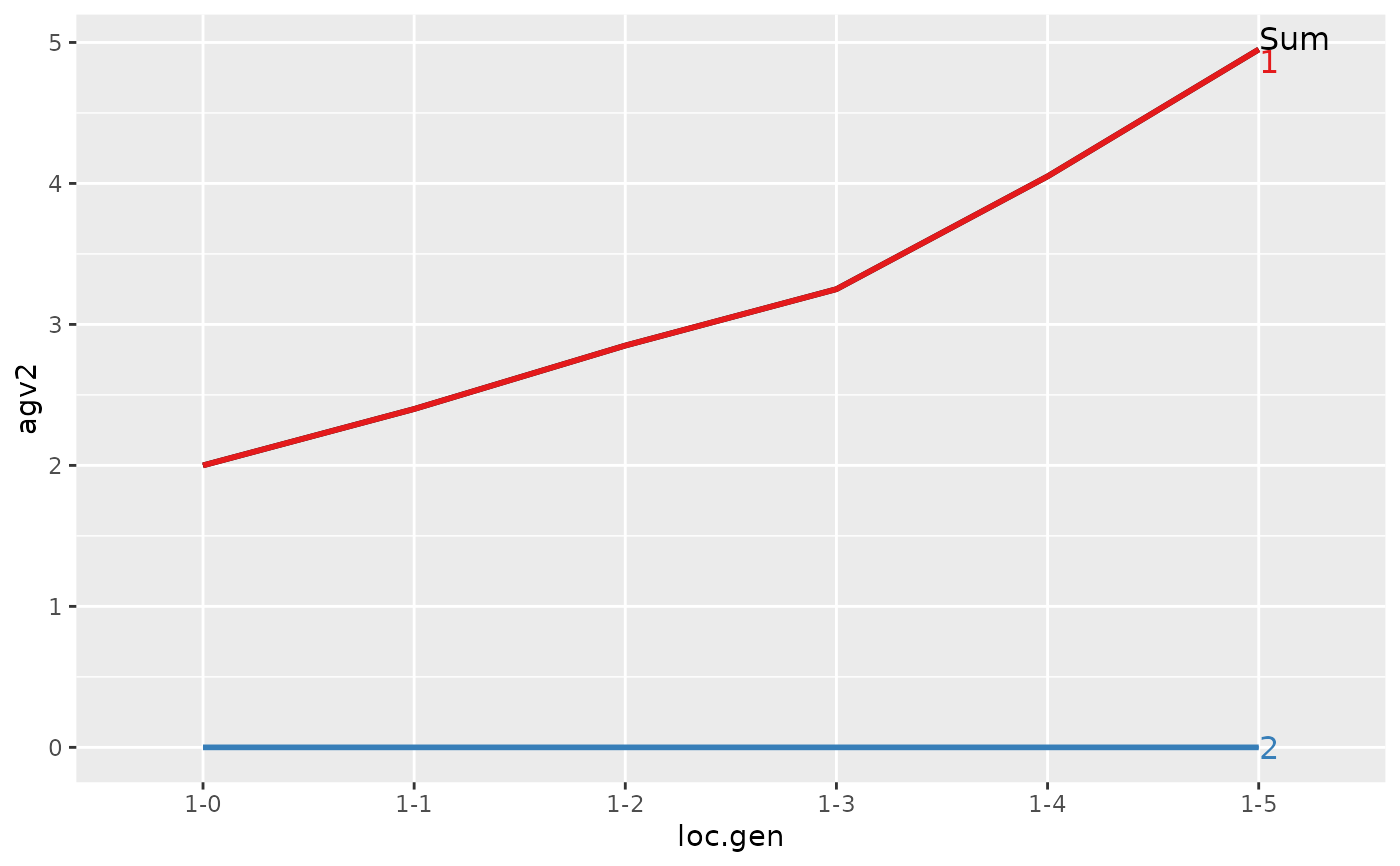
#> > ## Summarize and plot location specific trends
#> > (ret <- summary(res, by="loc.gen"))
#>
#>
#> Summary of partitions of breeding values
#> - paths: 2 (1, 2)
#> - traits: 2 (agv1, agv2)
#>
#> Trait: agv1
#>
#> loc.gen N Sum 1 2
#> 1 1-0 2 2.000 2.0000 0.0000
#> 2 1-1 2 2.400 2.4000 0.0000
#> 3 1-2 2 2.850 2.8500 0.0000
#> 4 1-3 2 3.250 3.2500 0.0000
#> 5 1-4 2 4.050 4.0500 0.0000
#> 6 1-5 2 4.950 4.9500 0.0000
#> 7 2-0 2 0.000 0.0000 0.0000
#> 8 2-1 2 -0.200 0.0000 -0.2000
#> 9 2-2 2 1.000 1.1000 -0.1000
#> 10 2-3 2 1.850 1.9000 -0.0500
#> 11 2-4 2 2.500 2.4250 0.0750
#> 12 2-5 2 3.325 3.2375 0.0875
#>
#> Trait: agv2
#>
#> loc.gen N Sum 1 2
#> 1 1-0 2 2.0000 2.0000 0.000
#> 2 1-1 2 2.4000 2.4000 0.000
#> 3 1-2 2 2.8500 2.8500 0.000
#> 4 1-3 2 3.2500 3.2500 0.000
#> 5 1-4 2 4.0500 4.0500 0.000
#> 6 1-5 2 4.9500 4.9500 0.000
#> 7 2-0 2 0.0000 0.0000 0.000
#> 8 2-1 2 0.4000 0.0000 0.400
#> 9 2-2 2 1.5000 1.1000 0.400
#> 10 2-3 2 2.4000 1.9000 0.500
#> 11 2-4 2 2.8750 2.4250 0.450
#> 12 2-5 2 3.7125 3.2375 0.475
#>
#>
#> > plot(ret)
 #>
#> > ## Summarize and plot location specific trends but only for location 1
#> > (ret <- summary(res, by="loc.gen", subset=res[[1]]$loc == 1))
#>
#>
#> Summary of partitions of breeding values
#> - paths: 2 (1, 2)
#> - traits: 2 (agv1, agv2)
#>
#> Trait: agv1
#>
#> loc.gen N Sum 1 2
#> 1 1-0 2 2.00 2.00 0
#> 2 1-1 2 2.40 2.40 0
#> 3 1-2 2 2.85 2.85 0
#> 4 1-3 2 3.25 3.25 0
#> 5 1-4 2 4.05 4.05 0
#> 6 1-5 2 4.95 4.95 0
#>
#> Trait: agv2
#>
#> loc.gen N Sum 1 2
#> 1 1-0 2 2.00 2.00 0
#> 2 1-1 2 2.40 2.40 0
#> 3 1-2 2 2.85 2.85 0
#> 4 1-3 2 3.25 3.25 0
#> 5 1-4 2 4.05 4.05 0
#> 6 1-5 2 4.95 4.95 0
#>
#>
#> > plot(ret)
#>
#> > ## Summarize and plot location specific trends but only for location 1
#> > (ret <- summary(res, by="loc.gen", subset=res[[1]]$loc == 1))
#>
#>
#> Summary of partitions of breeding values
#> - paths: 2 (1, 2)
#> - traits: 2 (agv1, agv2)
#>
#> Trait: agv1
#>
#> loc.gen N Sum 1 2
#> 1 1-0 2 2.00 2.00 0
#> 2 1-1 2 2.40 2.40 0
#> 3 1-2 2 2.85 2.85 0
#> 4 1-3 2 3.25 3.25 0
#> 5 1-4 2 4.05 4.05 0
#> 6 1-5 2 4.95 4.95 0
#>
#> Trait: agv2
#>
#> loc.gen N Sum 1 2
#> 1 1-0 2 2.00 2.00 0
#> 2 1-1 2 2.40 2.40 0
#> 3 1-2 2 2.85 2.85 0
#> 4 1-3 2 3.25 3.25 0
#> 5 1-4 2 4.05 4.05 0
#> 6 1-5 2 4.95 4.95 0
#>
#>
#> > plot(ret)

 #>
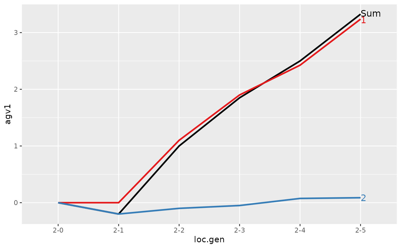
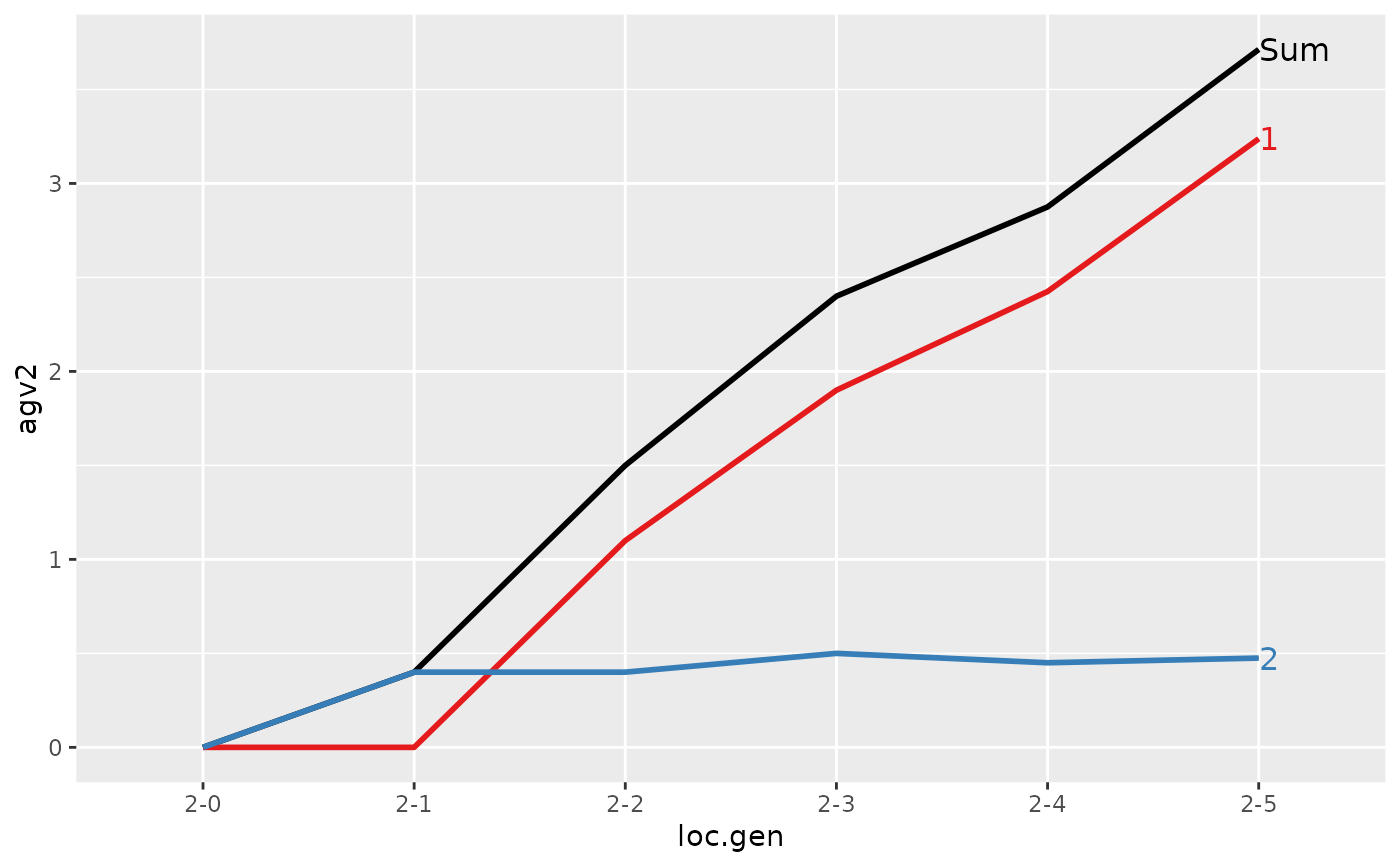
#> > ## Summarize and plot location specific trends but only for location 2
#> > (ret <- summary(res, by="loc.gen", subset=res[[1]]$loc == 2))
#>
#>
#> Summary of partitions of breeding values
#> - paths: 2 (1, 2)
#> - traits: 2 (agv1, agv2)
#>
#> Trait: agv1
#>
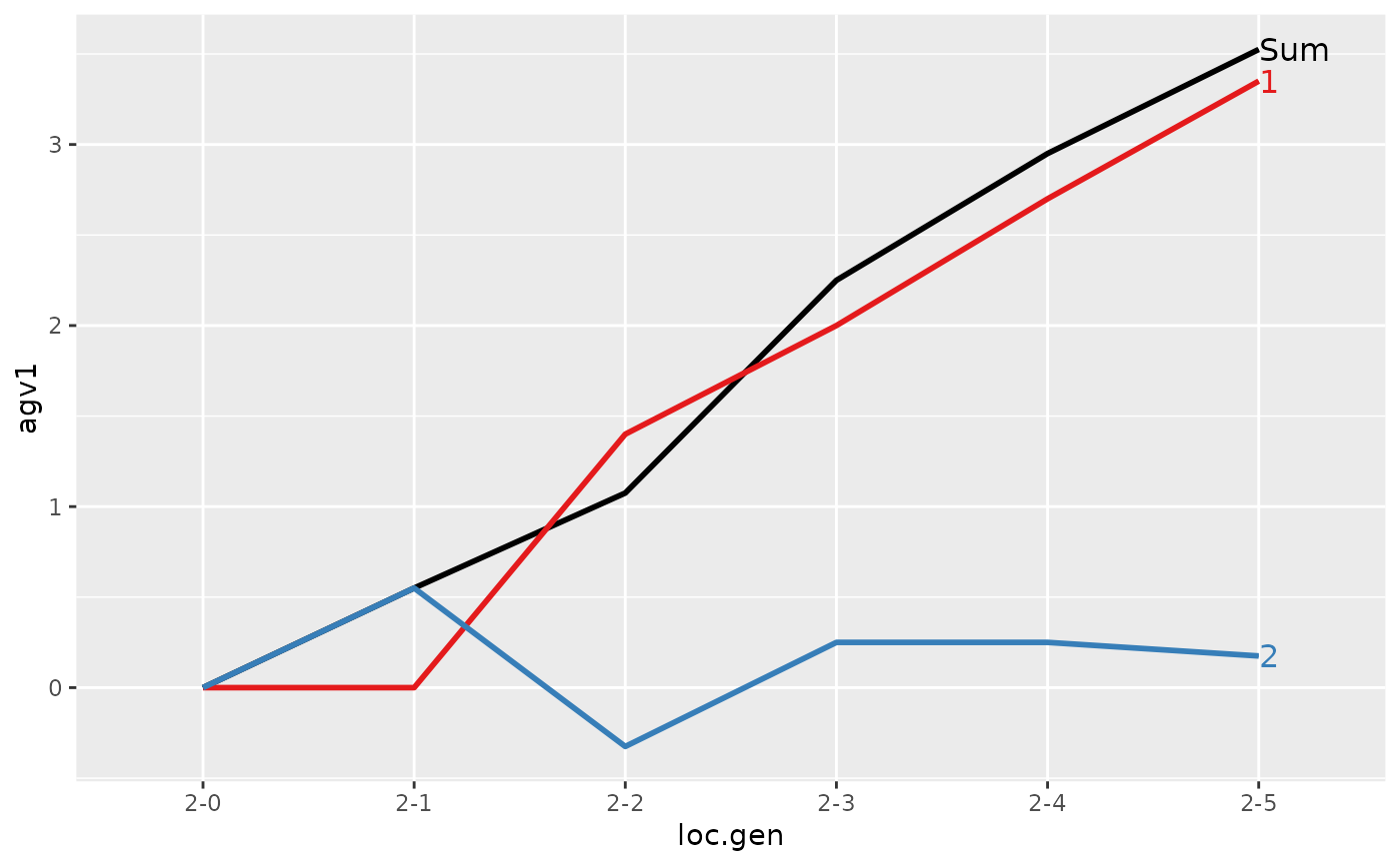
#> loc.gen N Sum 1 2
#> 1 2-0 2 0.000 0.0000 0.0000
#> 2 2-1 2 -0.200 0.0000 -0.2000
#> 3 2-2 2 1.000 1.1000 -0.1000
#> 4 2-3 2 1.850 1.9000 -0.0500
#> 5 2-4 2 2.500 2.4250 0.0750
#> 6 2-5 2 3.325 3.2375 0.0875
#>
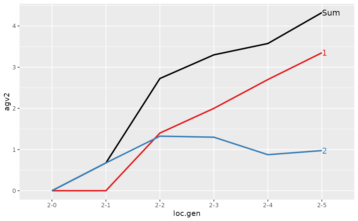
#> Trait: agv2
#>
#> loc.gen N Sum 1 2
#> 1 2-0 2 0.0000 0.0000 0.000
#> 2 2-1 2 0.4000 0.0000 0.400
#> 3 2-2 2 1.5000 1.1000 0.400
#> 4 2-3 2 2.4000 1.9000 0.500
#> 5 2-4 2 2.8750 2.4250 0.450
#> 6 2-5 2 3.7125 3.2375 0.475
#>
#>
#> > plot(ret)
#>
#> > ## Summarize and plot location specific trends but only for location 2
#> > (ret <- summary(res, by="loc.gen", subset=res[[1]]$loc == 2))
#>
#>
#> Summary of partitions of breeding values
#> - paths: 2 (1, 2)
#> - traits: 2 (agv1, agv2)
#>
#> Trait: agv1
#>
#> loc.gen N Sum 1 2
#> 1 2-0 2 0.000 0.0000 0.0000
#> 2 2-1 2 -0.200 0.0000 -0.2000
#> 3 2-2 2 1.000 1.1000 -0.1000
#> 4 2-3 2 1.850 1.9000 -0.0500
#> 5 2-4 2 2.500 2.4250 0.0750
#> 6 2-5 2 3.325 3.2375 0.0875
#>
#> Trait: agv2
#>
#> loc.gen N Sum 1 2
#> 1 2-0 2 0.0000 0.0000 0.000
#> 2 2-1 2 0.4000 0.0000 0.400
#> 3 2-2 2 1.5000 1.1000 0.400
#> 4 2-3 2 2.4000 1.9000 0.500
#> 5 2-4 2 2.8750 2.4250 0.450
#> 6 2-5 2 3.7125 3.2375 0.475
#>
#>
#> > plot(ret)
 #>
#> > ## Compute partitions by location and sex
#> > ped$loc.sex <- with(ped, paste(loc, sex, sep="-"))
#>
#> > (res <- AlphaPart(x=ped, colPath="loc.sex", colBV=c("agv1", "agv2")))
#>
#> Size:
#> - individuals: 24
#> - traits: 2 (agv1, agv2)
#> - paths: 4 (1-1, 1-2, 2-1, 2-2)
#> - unknown (missing) values:
#> agv1 agv2
#> 0 0
#>
#>
#> Partitions of breeding values
#> - individuals: 24
#> - paths: 4 (1-1, 1-2, 2-1, 2-2)
#> - traits: 2 (agv1, agv2)
#>
#> Trait: agv1
#>
#> id fid mid loc gen w1 w2 sex loc.gen pa1 pa2 loc.sex agv1 agv1_pa agv1_w agv1_1-1 agv1_1-2 agv1_2-1 agv1_2-2
#> 1 01 <NA> <NA> 1 0 2.0 2.0 1 1-0 0 0 1-1 2.0 0 2.0 2.0 0.0 0 0
#> 2 02 <NA> <NA> 1 0 2.0 2.0 2 1-0 0 0 1-2 2.0 0 2.0 0.0 2.0 0 0
#> 3 03 <NA> <NA> 2 0 0.0 0.0 1 2-0 0 0 2-1 0.0 0 0.0 0.0 0.0 0 0
#> 4 04 <NA> <NA> 2 0 0.0 0.0 2 2-0 0 0 2-2 0.0 0 0.0 0.0 0.0 0 0
#> 5 11 01 02 1 1 0.6 0.6 2 1-1 2 2 1-2 2.6 2 0.6 1.0 1.6 0 0
#> 6 12 01 02 1 1 0.2 0.2 1 1-1 2 2 1-1 2.2 2 0.2 1.2 1.0 0 0
#> ...
#> id fid mid loc gen w1 w2 sex loc.gen pa1 pa2 loc.sex agv1 agv1_pa agv1_w agv1_1-1 agv1_1-2 agv1_2-1 agv1_2-2
#> 19 43 32 33 2 4 -0.1 0.1 2 2-4 2.15 2.700 2-2 2.05 2.15 -0.1 1.1750 1.25 0 -0.3750
#> 20 44 32 34 2 4 0.3 0.3 2 2-4 2.65 2.650 2-2 2.95 2.65 0.3 1.1750 1.25 0 0.5250
#> 21 51 42 41 1 5 0.8 0.8 2 1-5 4.05 4.050 1-2 4.85 4.05 0.8 1.7000 3.15 0 0.0000
#> 22 52 42 41 1 5 1.0 1.0 2 1-5 4.05 4.050 1-2 5.05 4.05 1.0 1.7000 3.35 0 0.0000
#> 23 53 42 43 2 5 -0.2 0.2 2 2-5 3.05 3.425 2-2 2.85 3.05 -0.2 1.6375 1.60 0 -0.3875
#> 24 54 42 44 2 5 0.3 0.3 2 2-5 3.50 3.500 2-2 3.80 3.50 0.3 1.6375 1.60 0 0.5625
#>
#> Trait: agv2
#>
#> id fid mid loc gen w1 w2 sex loc.gen pa1 pa2 loc.sex agv2 agv2_pa agv2_w agv2_1-1 agv2_1-2 agv2_2-1 agv2_2-2
#> 1 01 <NA> <NA> 1 0 2.0 2.0 1 1-0 0 0 1-1 2.0 0 2.0 2.0 0.0 0 0
#> 2 02 <NA> <NA> 1 0 2.0 2.0 2 1-0 0 0 1-2 2.0 0 2.0 0.0 2.0 0 0
#> 3 03 <NA> <NA> 2 0 0.0 0.0 1 2-0 0 0 2-1 0.0 0 0.0 0.0 0.0 0 0
#> 4 04 <NA> <NA> 2 0 0.0 0.0 2 2-0 0 0 2-2 0.0 0 0.0 0.0 0.0 0 0
#> 5 11 01 02 1 1 0.6 0.6 2 1-1 2 2 1-2 2.6 2 0.6 1.0 1.6 0 0
#> 6 12 01 02 1 1 0.2 0.2 1 1-1 2 2 1-1 2.2 2 0.2 1.2 1.0 0 0
#> ...
#> id fid mid loc gen w1 w2 sex loc.gen pa1 pa2 loc.sex agv2 agv2_pa agv2_w agv2_1-1 agv2_1-2 agv2_2-1 agv2_2-2
#> 19 43 32 33 2 4 -0.1 0.1 2 2-4 2.15 2.700 2-2 2.800 2.700 0.1 1.1750 1.25 0 0.3750
#> 20 44 32 34 2 4 0.3 0.3 2 2-4 2.65 2.650 2-2 2.950 2.650 0.3 1.1750 1.25 0 0.5250
#> 21 51 42 41 1 5 0.8 0.8 2 1-5 4.05 4.050 1-2 4.850 4.050 0.8 1.7000 3.15 0 0.0000
#> 22 52 42 41 1 5 1.0 1.0 2 1-5 4.05 4.050 1-2 5.050 4.050 1.0 1.7000 3.35 0 0.0000
#> 23 53 42 43 2 5 -0.2 0.2 2 2-5 3.05 3.425 2-2 3.625 3.425 0.2 1.6375 1.60 0 0.3875
#> 24 54 42 44 2 5 0.3 0.3 2 2-5 3.50 3.500 2-2 3.800 3.500 0.3 1.6375 1.60 0 0.5625
#>
#>
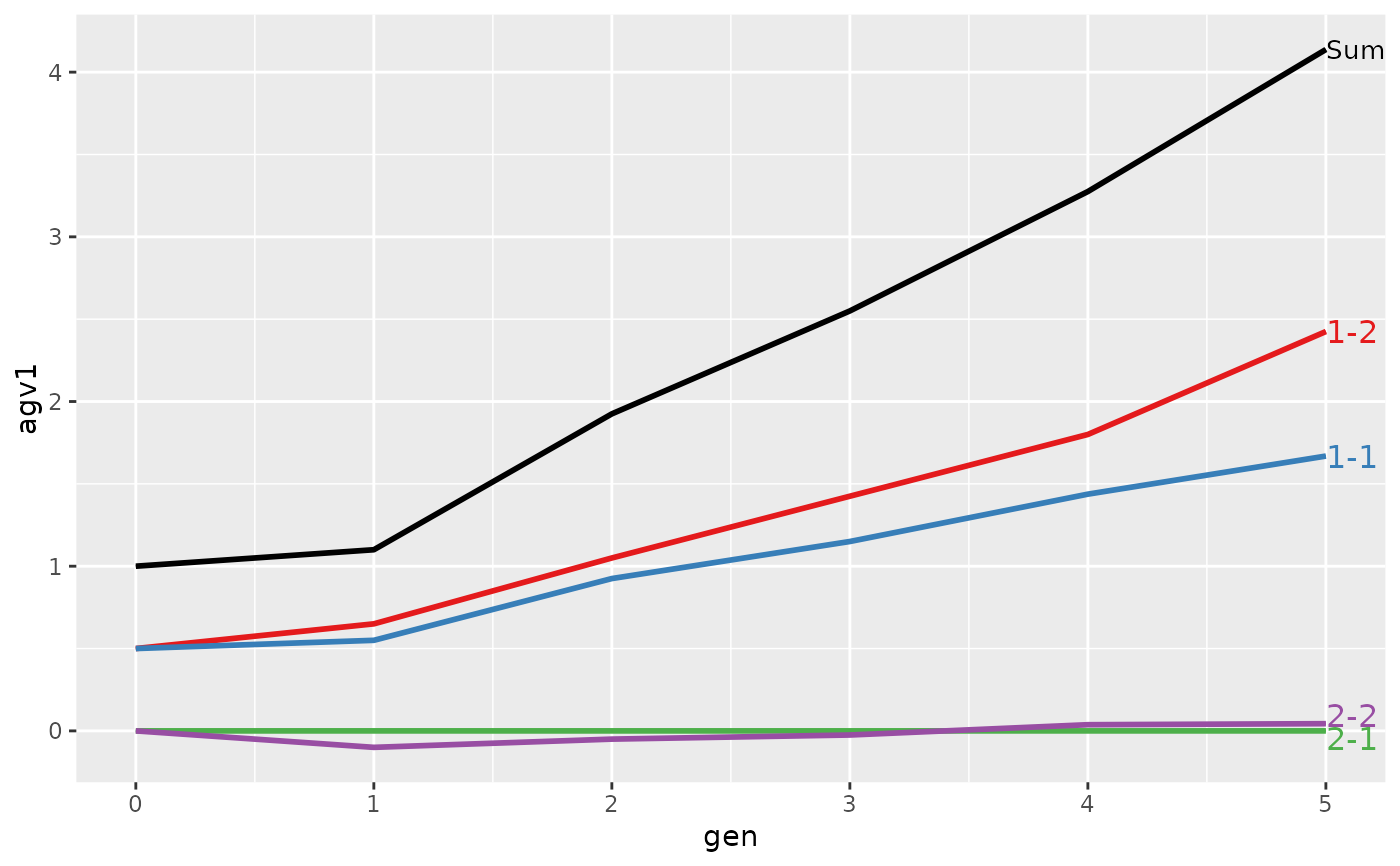
#> > ## Summarize and plot by generation (=trend)
#> > (ret <- summary(res, by="gen"))
#>
#>
#> Summary of partitions of breeding values
#> - paths: 4 (1-1, 1-2, 2-1, 2-2)
#> - traits: 2 (agv1, agv2)
#>
#> Trait: agv1
#>
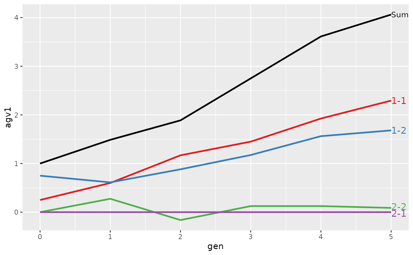
#> gen N Sum 1-1 1-2 2-1 2-2
#> 1 0 4 1.0000 0.50000 0.500 0 0.00000
#> 2 1 4 1.1000 0.55000 0.650 0 -0.10000
#> 3 2 4 1.9250 0.92500 1.050 0 -0.05000
#> 4 3 4 2.5500 1.15000 1.425 0 -0.02500
#> 5 4 4 3.2750 1.43750 1.800 0 0.03750
#> 6 5 4 4.1375 1.66875 2.425 0 0.04375
#>
#> Trait: agv2
#>
#> gen N Sum 1-1 1-2 2-1 2-2
#> 1 0 4 1.00000 0.50000 0.500 0 0.0000
#> 2 1 4 1.40000 0.55000 0.650 0 0.2000
#> 3 2 4 2.17500 0.92500 1.050 0 0.2000
#> 4 3 4 2.82500 1.15000 1.425 0 0.2500
#> 5 4 4 3.46250 1.43750 1.800 0 0.2250
#> 6 5 4 4.33125 1.66875 2.425 0 0.2375
#>
#>
#> > plot(ret)
#>
#> > ## Compute partitions by location and sex
#> > ped$loc.sex <- with(ped, paste(loc, sex, sep="-"))
#>
#> > (res <- AlphaPart(x=ped, colPath="loc.sex", colBV=c("agv1", "agv2")))
#>
#> Size:
#> - individuals: 24
#> - traits: 2 (agv1, agv2)
#> - paths: 4 (1-1, 1-2, 2-1, 2-2)
#> - unknown (missing) values:
#> agv1 agv2
#> 0 0
#>
#>
#> Partitions of breeding values
#> - individuals: 24
#> - paths: 4 (1-1, 1-2, 2-1, 2-2)
#> - traits: 2 (agv1, agv2)
#>
#> Trait: agv1
#>
#> id fid mid loc gen w1 w2 sex loc.gen pa1 pa2 loc.sex agv1 agv1_pa agv1_w agv1_1-1 agv1_1-2 agv1_2-1 agv1_2-2
#> 1 01 <NA> <NA> 1 0 2.0 2.0 1 1-0 0 0 1-1 2.0 0 2.0 2.0 0.0 0 0
#> 2 02 <NA> <NA> 1 0 2.0 2.0 2 1-0 0 0 1-2 2.0 0 2.0 0.0 2.0 0 0
#> 3 03 <NA> <NA> 2 0 0.0 0.0 1 2-0 0 0 2-1 0.0 0 0.0 0.0 0.0 0 0
#> 4 04 <NA> <NA> 2 0 0.0 0.0 2 2-0 0 0 2-2 0.0 0 0.0 0.0 0.0 0 0
#> 5 11 01 02 1 1 0.6 0.6 2 1-1 2 2 1-2 2.6 2 0.6 1.0 1.6 0 0
#> 6 12 01 02 1 1 0.2 0.2 1 1-1 2 2 1-1 2.2 2 0.2 1.2 1.0 0 0
#> ...
#> id fid mid loc gen w1 w2 sex loc.gen pa1 pa2 loc.sex agv1 agv1_pa agv1_w agv1_1-1 agv1_1-2 agv1_2-1 agv1_2-2
#> 19 43 32 33 2 4 -0.1 0.1 2 2-4 2.15 2.700 2-2 2.05 2.15 -0.1 1.1750 1.25 0 -0.3750
#> 20 44 32 34 2 4 0.3 0.3 2 2-4 2.65 2.650 2-2 2.95 2.65 0.3 1.1750 1.25 0 0.5250
#> 21 51 42 41 1 5 0.8 0.8 2 1-5 4.05 4.050 1-2 4.85 4.05 0.8 1.7000 3.15 0 0.0000
#> 22 52 42 41 1 5 1.0 1.0 2 1-5 4.05 4.050 1-2 5.05 4.05 1.0 1.7000 3.35 0 0.0000
#> 23 53 42 43 2 5 -0.2 0.2 2 2-5 3.05 3.425 2-2 2.85 3.05 -0.2 1.6375 1.60 0 -0.3875
#> 24 54 42 44 2 5 0.3 0.3 2 2-5 3.50 3.500 2-2 3.80 3.50 0.3 1.6375 1.60 0 0.5625
#>
#> Trait: agv2
#>
#> id fid mid loc gen w1 w2 sex loc.gen pa1 pa2 loc.sex agv2 agv2_pa agv2_w agv2_1-1 agv2_1-2 agv2_2-1 agv2_2-2
#> 1 01 <NA> <NA> 1 0 2.0 2.0 1 1-0 0 0 1-1 2.0 0 2.0 2.0 0.0 0 0
#> 2 02 <NA> <NA> 1 0 2.0 2.0 2 1-0 0 0 1-2 2.0 0 2.0 0.0 2.0 0 0
#> 3 03 <NA> <NA> 2 0 0.0 0.0 1 2-0 0 0 2-1 0.0 0 0.0 0.0 0.0 0 0
#> 4 04 <NA> <NA> 2 0 0.0 0.0 2 2-0 0 0 2-2 0.0 0 0.0 0.0 0.0 0 0
#> 5 11 01 02 1 1 0.6 0.6 2 1-1 2 2 1-2 2.6 2 0.6 1.0 1.6 0 0
#> 6 12 01 02 1 1 0.2 0.2 1 1-1 2 2 1-1 2.2 2 0.2 1.2 1.0 0 0
#> ...
#> id fid mid loc gen w1 w2 sex loc.gen pa1 pa2 loc.sex agv2 agv2_pa agv2_w agv2_1-1 agv2_1-2 agv2_2-1 agv2_2-2
#> 19 43 32 33 2 4 -0.1 0.1 2 2-4 2.15 2.700 2-2 2.800 2.700 0.1 1.1750 1.25 0 0.3750
#> 20 44 32 34 2 4 0.3 0.3 2 2-4 2.65 2.650 2-2 2.950 2.650 0.3 1.1750 1.25 0 0.5250
#> 21 51 42 41 1 5 0.8 0.8 2 1-5 4.05 4.050 1-2 4.850 4.050 0.8 1.7000 3.15 0 0.0000
#> 22 52 42 41 1 5 1.0 1.0 2 1-5 4.05 4.050 1-2 5.050 4.050 1.0 1.7000 3.35 0 0.0000
#> 23 53 42 43 2 5 -0.2 0.2 2 2-5 3.05 3.425 2-2 3.625 3.425 0.2 1.6375 1.60 0 0.3875
#> 24 54 42 44 2 5 0.3 0.3 2 2-5 3.50 3.500 2-2 3.800 3.500 0.3 1.6375 1.60 0 0.5625
#>
#>
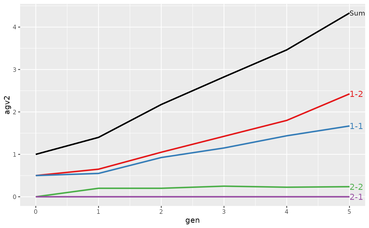
#> > ## Summarize and plot by generation (=trend)
#> > (ret <- summary(res, by="gen"))
#>
#>
#> Summary of partitions of breeding values
#> - paths: 4 (1-1, 1-2, 2-1, 2-2)
#> - traits: 2 (agv1, agv2)
#>
#> Trait: agv1
#>
#> gen N Sum 1-1 1-2 2-1 2-2
#> 1 0 4 1.0000 0.50000 0.500 0 0.00000
#> 2 1 4 1.1000 0.55000 0.650 0 -0.10000
#> 3 2 4 1.9250 0.92500 1.050 0 -0.05000
#> 4 3 4 2.5500 1.15000 1.425 0 -0.02500
#> 5 4 4 3.2750 1.43750 1.800 0 0.03750
#> 6 5 4 4.1375 1.66875 2.425 0 0.04375
#>
#> Trait: agv2
#>
#> gen N Sum 1-1 1-2 2-1 2-2
#> 1 0 4 1.00000 0.50000 0.500 0 0.0000
#> 2 1 4 1.40000 0.55000 0.650 0 0.2000
#> 3 2 4 2.17500 0.92500 1.050 0 0.2000
#> 4 3 4 2.82500 1.15000 1.425 0 0.2500
#> 5 4 4 3.46250 1.43750 1.800 0 0.2250
#> 6 5 4 4.33125 1.66875 2.425 0 0.2375
#>
#>
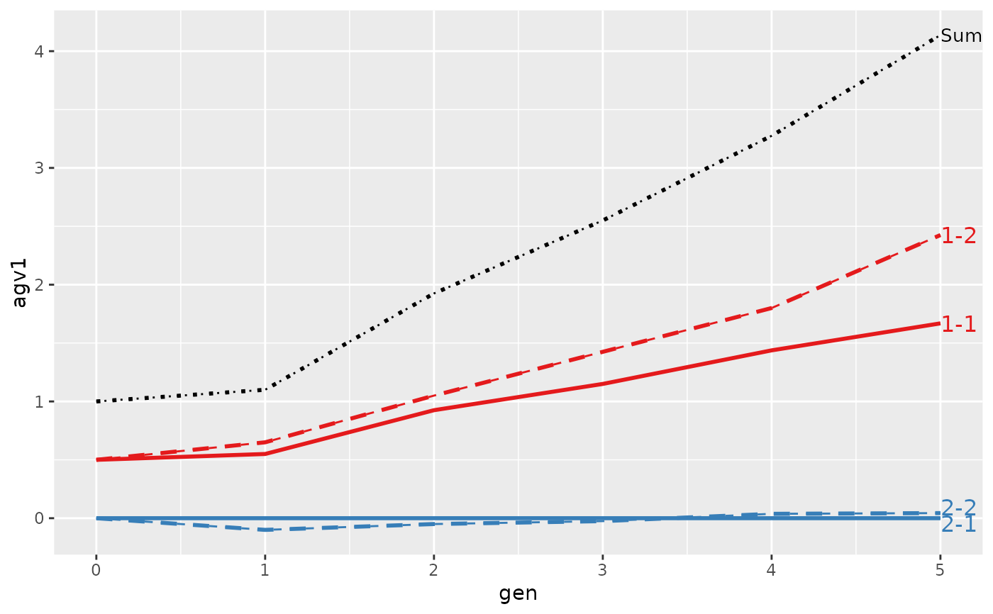
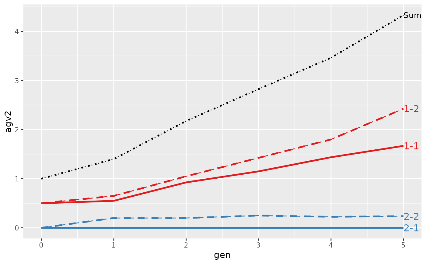
#> > plot(ret)
 #>
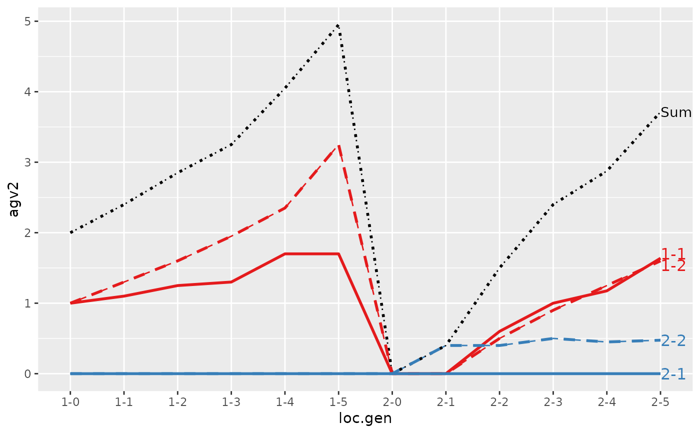
#> > plot(ret, lineTypeList=list("-1"=1, "-2"=2, def=3))
#>
#> > plot(ret, lineTypeList=list("-1"=1, "-2"=2, def=3))
 #>
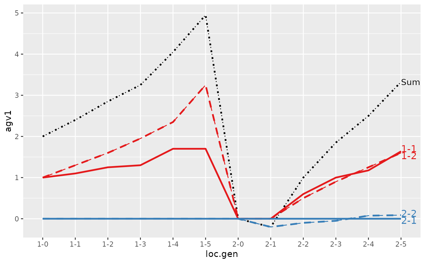
#> > ## Summarize and plot location specific trends
#> > (ret <- summary(res, by="loc.gen"))
#>
#>
#> Summary of partitions of breeding values
#> - paths: 4 (1-1, 1-2, 2-1, 2-2)
#> - traits: 2 (agv1, agv2)
#>
#> Trait: agv1
#>
#> loc.gen N Sum 1-1 1-2 2-1 2-2
#> 1 1-0 2 2.000 1.0000 1.00 0 0.0000
#> 2 1-1 2 2.400 1.1000 1.30 0 0.0000
#> 3 1-2 2 2.850 1.2500 1.60 0 0.0000
#> 4 1-3 2 3.250 1.3000 1.95 0 0.0000
#> 5 1-4 2 4.050 1.7000 2.35 0 0.0000
#> 6 1-5 2 4.950 1.7000 3.25 0 0.0000
#> 7 2-0 2 0.000 0.0000 0.00 0 0.0000
#> 8 2-1 2 -0.200 0.0000 0.00 0 -0.2000
#> 9 2-2 2 1.000 0.6000 0.50 0 -0.1000
#> 10 2-3 2 1.850 1.0000 0.90 0 -0.0500
#> 11 2-4 2 2.500 1.1750 1.25 0 0.0750
#> 12 2-5 2 3.325 1.6375 1.60 0 0.0875
#>
#> Trait: agv2
#>
#> loc.gen N Sum 1-1 1-2 2-1 2-2
#> 1 1-0 2 2.0000 1.0000 1.00 0 0.000
#> 2 1-1 2 2.4000 1.1000 1.30 0 0.000
#> 3 1-2 2 2.8500 1.2500 1.60 0 0.000
#> 4 1-3 2 3.2500 1.3000 1.95 0 0.000
#> 5 1-4 2 4.0500 1.7000 2.35 0 0.000
#> 6 1-5 2 4.9500 1.7000 3.25 0 0.000
#> 7 2-0 2 0.0000 0.0000 0.00 0 0.000
#> 8 2-1 2 0.4000 0.0000 0.00 0 0.400
#> 9 2-2 2 1.5000 0.6000 0.50 0 0.400
#> 10 2-3 2 2.4000 1.0000 0.90 0 0.500
#> 11 2-4 2 2.8750 1.1750 1.25 0 0.450
#> 12 2-5 2 3.7125 1.6375 1.60 0 0.475
#>
#>
#> > plot(ret, lineTypeList=list("-1"=1, "-2"=2, def=3))
#>
#> > ## Summarize and plot location specific trends
#> > (ret <- summary(res, by="loc.gen"))
#>
#>
#> Summary of partitions of breeding values
#> - paths: 4 (1-1, 1-2, 2-1, 2-2)
#> - traits: 2 (agv1, agv2)
#>
#> Trait: agv1
#>
#> loc.gen N Sum 1-1 1-2 2-1 2-2
#> 1 1-0 2 2.000 1.0000 1.00 0 0.0000
#> 2 1-1 2 2.400 1.1000 1.30 0 0.0000
#> 3 1-2 2 2.850 1.2500 1.60 0 0.0000
#> 4 1-3 2 3.250 1.3000 1.95 0 0.0000
#> 5 1-4 2 4.050 1.7000 2.35 0 0.0000
#> 6 1-5 2 4.950 1.7000 3.25 0 0.0000
#> 7 2-0 2 0.000 0.0000 0.00 0 0.0000
#> 8 2-1 2 -0.200 0.0000 0.00 0 -0.2000
#> 9 2-2 2 1.000 0.6000 0.50 0 -0.1000
#> 10 2-3 2 1.850 1.0000 0.90 0 -0.0500
#> 11 2-4 2 2.500 1.1750 1.25 0 0.0750
#> 12 2-5 2 3.325 1.6375 1.60 0 0.0875
#>
#> Trait: agv2
#>
#> loc.gen N Sum 1-1 1-2 2-1 2-2
#> 1 1-0 2 2.0000 1.0000 1.00 0 0.000
#> 2 1-1 2 2.4000 1.1000 1.30 0 0.000
#> 3 1-2 2 2.8500 1.2500 1.60 0 0.000
#> 4 1-3 2 3.2500 1.3000 1.95 0 0.000
#> 5 1-4 2 4.0500 1.7000 2.35 0 0.000
#> 6 1-5 2 4.9500 1.7000 3.25 0 0.000
#> 7 2-0 2 0.0000 0.0000 0.00 0 0.000
#> 8 2-1 2 0.4000 0.0000 0.00 0 0.400
#> 9 2-2 2 1.5000 0.6000 0.50 0 0.400
#> 10 2-3 2 2.4000 1.0000 0.90 0 0.500
#> 11 2-4 2 2.8750 1.1750 1.25 0 0.450
#> 12 2-5 2 3.7125 1.6375 1.60 0 0.475
#>
#>
#> > plot(ret, lineTypeList=list("-1"=1, "-2"=2, def=3))
 #>
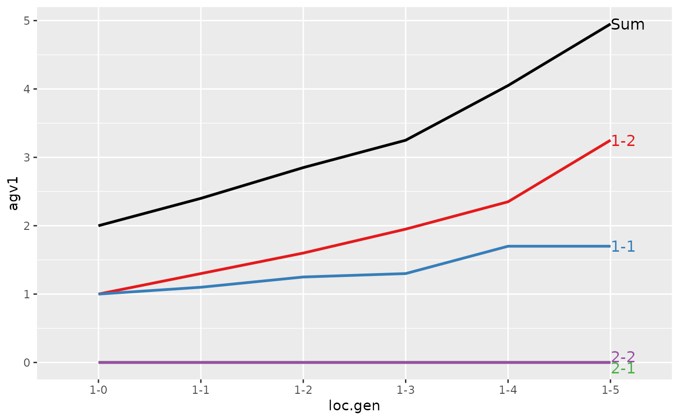
#> > ## Summarize and plot location specific trends but only for location 1
#> > (ret <- summary(res, by="loc.gen", subset=res[[1]]$loc == 1))
#>
#>
#> Summary of partitions of breeding values
#> - paths: 4 (1-1, 1-2, 2-1, 2-2)
#> - traits: 2 (agv1, agv2)
#>
#> Trait: agv1
#>
#> loc.gen N Sum 1-1 1-2 2-1 2-2
#> 1 1-0 2 2.00 1.00 1.00 0 0
#> 2 1-1 2 2.40 1.10 1.30 0 0
#> 3 1-2 2 2.85 1.25 1.60 0 0
#> 4 1-3 2 3.25 1.30 1.95 0 0
#> 5 1-4 2 4.05 1.70 2.35 0 0
#> 6 1-5 2 4.95 1.70 3.25 0 0
#>
#> Trait: agv2
#>
#> loc.gen N Sum 1-1 1-2 2-1 2-2
#> 1 1-0 2 2.00 1.00 1.00 0 0
#> 2 1-1 2 2.40 1.10 1.30 0 0
#> 3 1-2 2 2.85 1.25 1.60 0 0
#> 4 1-3 2 3.25 1.30 1.95 0 0
#> 5 1-4 2 4.05 1.70 2.35 0 0
#> 6 1-5 2 4.95 1.70 3.25 0 0
#>
#>
#> > plot(ret)
#>
#> > ## Summarize and plot location specific trends but only for location 1
#> > (ret <- summary(res, by="loc.gen", subset=res[[1]]$loc == 1))
#>
#>
#> Summary of partitions of breeding values
#> - paths: 4 (1-1, 1-2, 2-1, 2-2)
#> - traits: 2 (agv1, agv2)
#>
#> Trait: agv1
#>
#> loc.gen N Sum 1-1 1-2 2-1 2-2
#> 1 1-0 2 2.00 1.00 1.00 0 0
#> 2 1-1 2 2.40 1.10 1.30 0 0
#> 3 1-2 2 2.85 1.25 1.60 0 0
#> 4 1-3 2 3.25 1.30 1.95 0 0
#> 5 1-4 2 4.05 1.70 2.35 0 0
#> 6 1-5 2 4.95 1.70 3.25 0 0
#>
#> Trait: agv2
#>
#> loc.gen N Sum 1-1 1-2 2-1 2-2
#> 1 1-0 2 2.00 1.00 1.00 0 0
#> 2 1-1 2 2.40 1.10 1.30 0 0
#> 3 1-2 2 2.85 1.25 1.60 0 0
#> 4 1-3 2 3.25 1.30 1.95 0 0
#> 5 1-4 2 4.05 1.70 2.35 0 0
#> 6 1-5 2 4.95 1.70 3.25 0 0
#>
#>
#> > plot(ret)
 #>
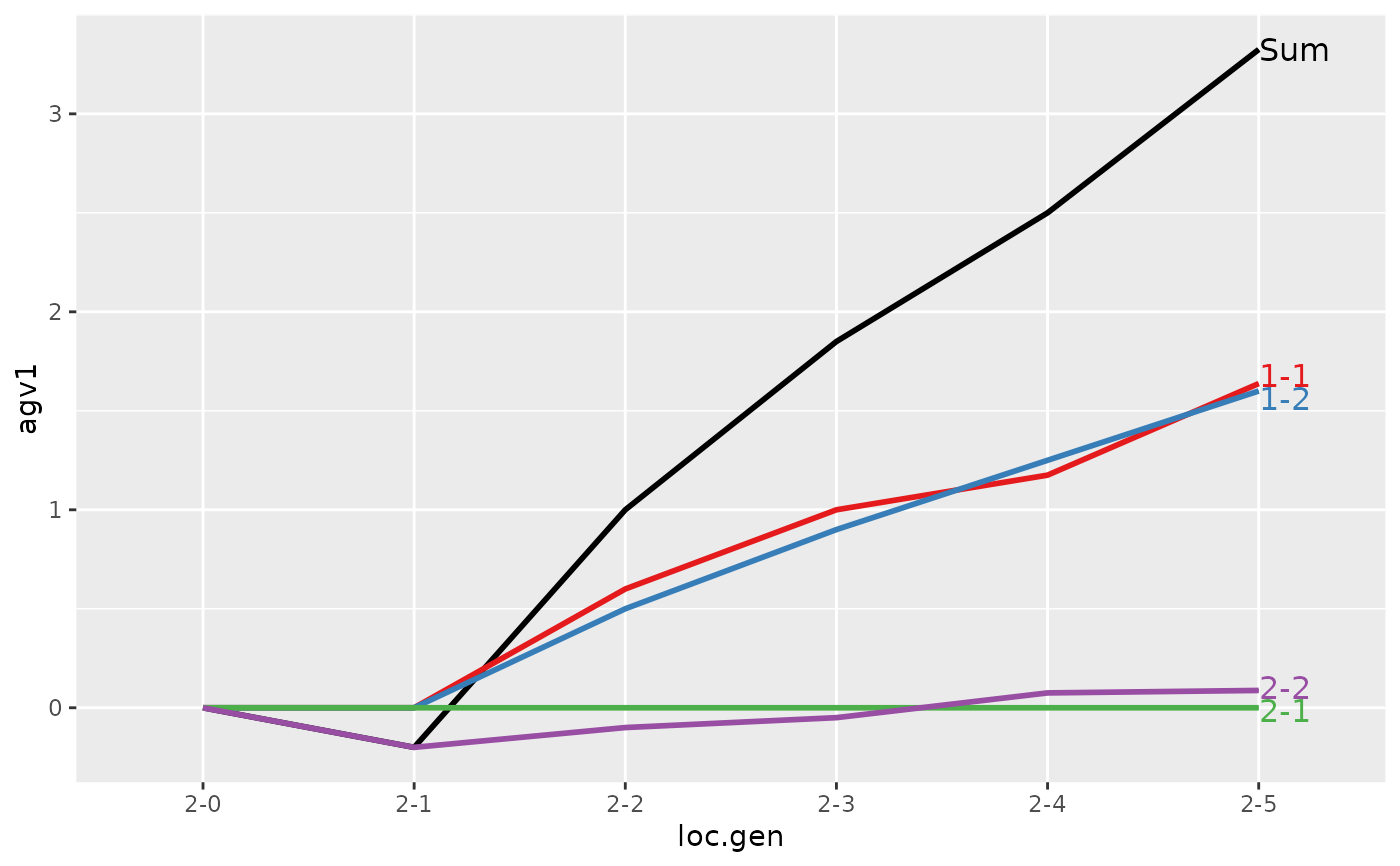
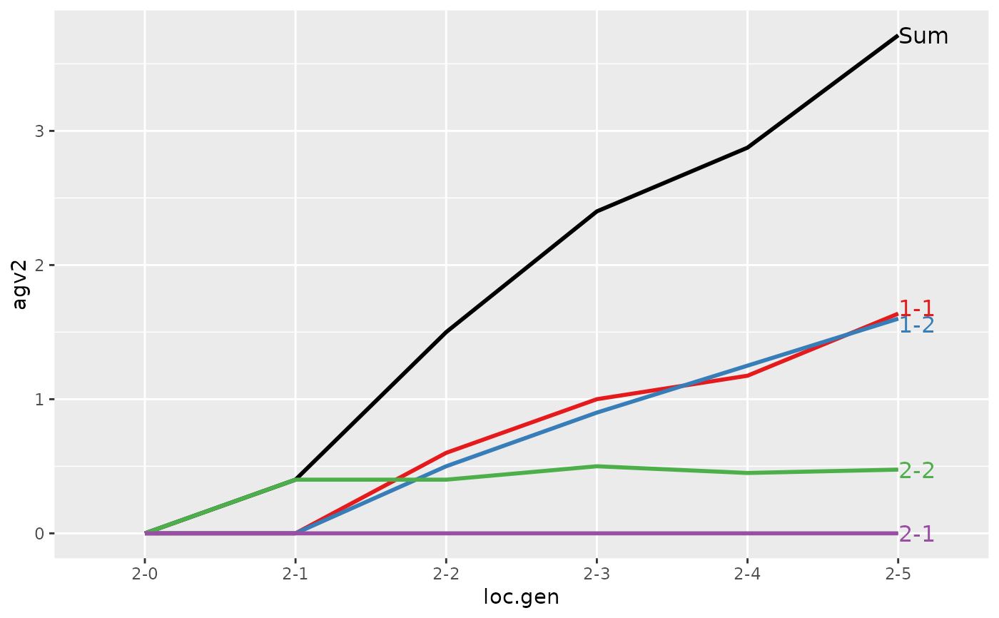
#> > ## Summarize and plot location specific trends but only for location 2
#> > (ret <- summary(res, by="loc.gen", subset=res[[1]]$loc == 2))
#>
#>
#> Summary of partitions of breeding values
#> - paths: 4 (1-1, 1-2, 2-1, 2-2)
#> - traits: 2 (agv1, agv2)
#>
#> Trait: agv1
#>
#> loc.gen N Sum 1-1 1-2 2-1 2-2
#> 1 2-0 2 0.000 0.0000 0.00 0 0.0000
#> 2 2-1 2 -0.200 0.0000 0.00 0 -0.2000
#> 3 2-2 2 1.000 0.6000 0.50 0 -0.1000
#> 4 2-3 2 1.850 1.0000 0.90 0 -0.0500
#> 5 2-4 2 2.500 1.1750 1.25 0 0.0750
#> 6 2-5 2 3.325 1.6375 1.60 0 0.0875
#>
#> Trait: agv2
#>
#> loc.gen N Sum 1-1 1-2 2-1 2-2
#> 1 2-0 2 0.0000 0.0000 0.00 0 0.000
#> 2 2-1 2 0.4000 0.0000 0.00 0 0.400
#> 3 2-2 2 1.5000 0.6000 0.50 0 0.400
#> 4 2-3 2 2.4000 1.0000 0.90 0 0.500
#> 5 2-4 2 2.8750 1.1750 1.25 0 0.450
#> 6 2-5 2 3.7125 1.6375 1.60 0 0.475
#>
#>
#> > plot(ret)
#>
#> > ## Summarize and plot location specific trends but only for location 2
#> > (ret <- summary(res, by="loc.gen", subset=res[[1]]$loc == 2))
#>
#>
#> Summary of partitions of breeding values
#> - paths: 4 (1-1, 1-2, 2-1, 2-2)
#> - traits: 2 (agv1, agv2)
#>
#> Trait: agv1
#>
#> loc.gen N Sum 1-1 1-2 2-1 2-2
#> 1 2-0 2 0.000 0.0000 0.00 0 0.0000
#> 2 2-1 2 -0.200 0.0000 0.00 0 -0.2000
#> 3 2-2 2 1.000 0.6000 0.50 0 -0.1000
#> 4 2-3 2 1.850 1.0000 0.90 0 -0.0500
#> 5 2-4 2 2.500 1.1750 1.25 0 0.0750
#> 6 2-5 2 3.325 1.6375 1.60 0 0.0875
#>
#> Trait: agv2
#>
#> loc.gen N Sum 1-1 1-2 2-1 2-2
#> 1 2-0 2 0.0000 0.0000 0.00 0 0.000
#> 2 2-1 2 0.4000 0.0000 0.00 0 0.400
#> 3 2-2 2 1.5000 0.6000 0.50 0 0.400
#> 4 2-3 2 2.4000 1.0000 0.90 0 0.500
#> 5 2-4 2 2.8750 1.1750 1.25 0 0.450
#> 6 2-5 2 3.7125 1.6375 1.60 0 0.475
#>
#>
#> > plot(ret)
 #>
#> > ###-----------------------------------------------------------------------------
#> > ### AlphaPart_deterministic.R ends here
demo(topic="AlphaPart_stochastic", package="AlphaPart",
ask=interactive())
#>
#>
#> demo(AlphaPart_stochastic)
#> ---- ~~~~~~~~~~~~~~~~~~~~
#>
#> > ### demo_stohastic.R
#> > ###-----------------------------------------------------------------------------
#> > ### $Id$
#> > ###-----------------------------------------------------------------------------
#> >
#> > ### DESCRIPTION OF A DEMONSTRATION
#> > ###-----------------------------------------------------------------------------
#> >
#> > ## A demonstration with a simple example to see in action the partitioning of
#> > ## additive genetic values by paths (Garcia-Cortes et al., 2008; Animal)
#> > ##
#> > ## STOHASTIC SIMULATION (sort of)
#> > ##
#> > ## We have two locations (1 and 2). The first location has individualss with higher
#> > ## additive genetic value. Males from the first location are imported males to the
#> > ## second location from generation 2/3. This clearly leads to genetic gain in the
#> > ## second location. However, the second location can also perform their own selection
#> > ## so the question is how much genetic gain is due to the import of genes from the
#> > ## first location and due to their own selection.
#> > ##
#> > ## Above scenario will be tested with a simple example of a pedigree bellow. Two
#> > ## scenarios will be evaluated: without or with own selection in the second location.
#> > ## Selection will always be present in the first location.
#> > ##
#> > ## Additive genetic values are provided, i.e., no inference is being done!
#> > ##
#> > ## The idea of this example is not to do extensive simulations, but just to have
#> > ## a simple example to see how the partitioning of additive genetic values works.
#> >
#> > ### SETUP
#> > ###-----------------------------------------------------------------------------
#> >
#> > options(width=200)
#>
#> > ## install.packages(pkg=c("truncnorm"), dep=TRUE)
#> > library(package="truncnorm")
#>
#> > ### EXAMPLE PEDIGREE
#> > ###-----------------------------------------------------------------------------
#> >
#> > ## Generation 0
#> > id0 <- c("01", "02", "03", "04", "05", "06", "07", "08")
#>
#> > fid0 <- mid0 <- rep(NA, times=length(id0))
#>
#> > h0 <- rep(c(1, 2), each=4)
#>
#> > g0 <- rep(0, times=length(id0))
#>
#> > ## Generation 1
#> > id1 <- c("11", "12", "13", "14", "15", "16", "17", "18")
#>
#> > fid1 <- c("02", "02", "02", "02", "06", "06", "06", "06")
#>
#> > mid1 <- c("01", "01", "03", "04", "05", "05", "07", "08")
#>
#> > h1 <- h0
#>
#> > g1 <- rep(1, times=length(id1))
#>
#> > ## Generation 2
#> > id2 <- c("21", "22", "23", "24", "25", "26", "27", "28")
#>
#> > fid2 <- c("13", "13", "13", "13", "13", "13", "13", "13")
#>
#> > mid2 <- c("11", "12", "14", "14", "15", "16", "17", "18")
#>
#> > h2 <- h0
#>
#> > g2 <- rep(2, times=length(id2))
#>
#> > ## Generation 3
#> > id3 <- c("31", "32", "33", "34", "35", "36", "37", "38")
#>
#> > fid3 <- c("24", "24", "24", "24", "24", "24", "24", "24")
#>
#> > mid3 <- c("21", "21", "22", "23", "25", "26", "27", "28")
#>
#> > h3 <- h0
#>
#> > g3 <- rep(3, times=length(id3))
#>
#> > ## Generation 4
#> > id4 <- c("41", "42", "43", "44", "45", "46", "47", "48")
#>
#> > fid4 <- c("34", "34", "34", "34", "34", "34", "34", "34")
#>
#> > mid4 <- c("31", "32", "32", "33", "35", "36", "37", "38")
#>
#> > h4 <- h0
#>
#> > g4 <- rep(4, times=length(id4))
#>
#> > ## Generation 5
#> > id5 <- c("51", "52", "53", "54", "55", "56", "57", "58")
#>
#> > fid5 <- c("44", "44", "44", "44", "44", "44", "44", "44")
#>
#> > mid5 <- c("41", "42", "43", "43", "45", "46", "47", "48")
#>
#> > h5 <- h0
#>
#> > g5 <- rep(5, times=length(id4))
#>
#> > ped <- data.frame( id=c( id0, id1, id2, id3, id4, id5),
#> + fid=c(fid0, fid1, fid2, fid3, fid4, fid5),
#> + mid=c(mid0, mid1, mid2, mid3, mid4, mid5),
#> + loc=c( h0, h1, h2, h3, h4, h5),
#> + gen=c( g0, g1, g2, g3, g4, g5))
#>
#> > ped$sex <- 2
#>
#> > ped[ped$id %in% ped$fid, "sex"] <- 1
#>
#> > ped$loc.gen <- with(ped, paste(loc, gen, sep="-"))
#>
#> > ### SIMULATE ADDITIVE GENETIC VALUES - STOHASTIC
#> > ###-----------------------------------------------------------------------------
#> >
#> > ## --- Parameters of simulation ---
#> >
#> > ## Additive genetic mean in founders by location
#> > mu1 <- 2
#>
#> > mu2 <- 0
#>
#> > ## Additive genetic variance in population
#> > sigma2 <- 1
#>
#> > sigma <- sqrt(sigma2)
#>
#> > ## Threshold value for Mendelian sampling for selection - only values above this
#> > ## will be accepted in simulation
#> > t <- 0
#>
#> > ## Set seed for simulation
#> > set.seed(seed=19791123)
#>
#> > ## --- Start of simulation ---
#> >
#> > ped$agv1 <- NA ## Scenario (trait) 1: No selection in the second location
#>
#> > ped$agv2 <- NA ## Scenario (trait) 2: Selection in the second location
#>
#> > ## Generation 0 - founders (for simplicity set their values to the mean of location)
#> > ped[ped$gen == 0 & ped$loc == 1, c("agv1", "agv2")] <- mu1
#>
#> > ped[ped$gen == 0 & ped$loc == 2, c("agv1", "agv2")] <- mu2
#>
#> > ## Generation 1+ - non-founders
#> > for(i in (length(g0)+1):nrow(ped)) {
#> + ## Scenario (trait) 1: selection only in the first location
#> + if(ped[i, "loc"] == 1) {
#> + w <- rtruncnorm(n=1, mean=0, sd=sqrt(sigma2/2), a=t)
#> + } else {
#> + w <- rnorm(n=1, mean=0, sd=sqrt(sigma2/2))
#> + }
#> + ped[i, "agv1"] <- round(0.5 * ped[ped$id %in% ped[i, "fid"], "agv1"] +
#> + 0.5 * ped[ped$id %in% ped[i, "mid"], "agv1"] +
#> + w, digits=1)
#> + ## Scenario (trait) 2: selection in both locations
#> + if(ped[i, "loc"] == 2) {
#> + w <- rtruncnorm(n=1, mean=0, sd=sqrt(sigma2/2), a=t)
#> + } ## for location 1 take the same values as above
#> + ped[i, "agv2"] <- round(0.5 * ped[ped$id %in% ped[i, "fid"], "agv2"] +
#> + 0.5 * ped[ped$id %in% ped[i, "mid"], "agv2"] +
#> + w, digits=1)
#> + }
#>
#> > ### PLOT INDIVIDUAL ADDITIVE GENETIC VALUES
#> > ###-----------------------------------------------------------------------------
#> >
#> > par(mfrow=c(2, 1), bty="l", pty="m", mar=c(2, 2, 1, 1) + .1, mgp=c(0.7, 0.2, 0))
#>
#> > tmp <- ped$gen + c(-1.5, -0.5, 0.5, 1.5) * 0.1
#>
#> > with(ped, plot(agv1 ~ tmp, pch=c(19, 21)[ped$loc], ylab="Additive genetic value",
#> + xlab="Generation", main="Selection in location 1", axes=FALSE,
#> + ylim=range(c(agv1, agv2))))
#>
#> > axis(1, labels=FALSE, tick=FALSE); axis(2, labels=FALSE, tick=FALSE); box()
#>
#> > legend(x="topleft", legend=c(1, 2), title="Location", pch=c(19, 21), bty="n")
#>
#> > with(ped, plot(agv2 ~ tmp, pch=c(19, 21)[ped$loc], ylab="Additive genetic value",
#> + xlab="Generation", main="Selection in locations 1 and 2", axes=FALSE,
#> + ylim=range(c(agv1, agv2))))
#>
#> > ###-----------------------------------------------------------------------------
#> > ### AlphaPart_deterministic.R ends here
demo(topic="AlphaPart_stochastic", package="AlphaPart",
ask=interactive())
#>
#>
#> demo(AlphaPart_stochastic)
#> ---- ~~~~~~~~~~~~~~~~~~~~
#>
#> > ### demo_stohastic.R
#> > ###-----------------------------------------------------------------------------
#> > ### $Id$
#> > ###-----------------------------------------------------------------------------
#> >
#> > ### DESCRIPTION OF A DEMONSTRATION
#> > ###-----------------------------------------------------------------------------
#> >
#> > ## A demonstration with a simple example to see in action the partitioning of
#> > ## additive genetic values by paths (Garcia-Cortes et al., 2008; Animal)
#> > ##
#> > ## STOHASTIC SIMULATION (sort of)
#> > ##
#> > ## We have two locations (1 and 2). The first location has individualss with higher
#> > ## additive genetic value. Males from the first location are imported males to the
#> > ## second location from generation 2/3. This clearly leads to genetic gain in the
#> > ## second location. However, the second location can also perform their own selection
#> > ## so the question is how much genetic gain is due to the import of genes from the
#> > ## first location and due to their own selection.
#> > ##
#> > ## Above scenario will be tested with a simple example of a pedigree bellow. Two
#> > ## scenarios will be evaluated: without or with own selection in the second location.
#> > ## Selection will always be present in the first location.
#> > ##
#> > ## Additive genetic values are provided, i.e., no inference is being done!
#> > ##
#> > ## The idea of this example is not to do extensive simulations, but just to have
#> > ## a simple example to see how the partitioning of additive genetic values works.
#> >
#> > ### SETUP
#> > ###-----------------------------------------------------------------------------
#> >
#> > options(width=200)
#>
#> > ## install.packages(pkg=c("truncnorm"), dep=TRUE)
#> > library(package="truncnorm")
#>
#> > ### EXAMPLE PEDIGREE
#> > ###-----------------------------------------------------------------------------
#> >
#> > ## Generation 0
#> > id0 <- c("01", "02", "03", "04", "05", "06", "07", "08")
#>
#> > fid0 <- mid0 <- rep(NA, times=length(id0))
#>
#> > h0 <- rep(c(1, 2), each=4)
#>
#> > g0 <- rep(0, times=length(id0))
#>
#> > ## Generation 1
#> > id1 <- c("11", "12", "13", "14", "15", "16", "17", "18")
#>
#> > fid1 <- c("02", "02", "02", "02", "06", "06", "06", "06")
#>
#> > mid1 <- c("01", "01", "03", "04", "05", "05", "07", "08")
#>
#> > h1 <- h0
#>
#> > g1 <- rep(1, times=length(id1))
#>
#> > ## Generation 2
#> > id2 <- c("21", "22", "23", "24", "25", "26", "27", "28")
#>
#> > fid2 <- c("13", "13", "13", "13", "13", "13", "13", "13")
#>
#> > mid2 <- c("11", "12", "14", "14", "15", "16", "17", "18")
#>
#> > h2 <- h0
#>
#> > g2 <- rep(2, times=length(id2))
#>
#> > ## Generation 3
#> > id3 <- c("31", "32", "33", "34", "35", "36", "37", "38")
#>
#> > fid3 <- c("24", "24", "24", "24", "24", "24", "24", "24")
#>
#> > mid3 <- c("21", "21", "22", "23", "25", "26", "27", "28")
#>
#> > h3 <- h0
#>
#> > g3 <- rep(3, times=length(id3))
#>
#> > ## Generation 4
#> > id4 <- c("41", "42", "43", "44", "45", "46", "47", "48")
#>
#> > fid4 <- c("34", "34", "34", "34", "34", "34", "34", "34")
#>
#> > mid4 <- c("31", "32", "32", "33", "35", "36", "37", "38")
#>
#> > h4 <- h0
#>
#> > g4 <- rep(4, times=length(id4))
#>
#> > ## Generation 5
#> > id5 <- c("51", "52", "53", "54", "55", "56", "57", "58")
#>
#> > fid5 <- c("44", "44", "44", "44", "44", "44", "44", "44")
#>
#> > mid5 <- c("41", "42", "43", "43", "45", "46", "47", "48")
#>
#> > h5 <- h0
#>
#> > g5 <- rep(5, times=length(id4))
#>
#> > ped <- data.frame( id=c( id0, id1, id2, id3, id4, id5),
#> + fid=c(fid0, fid1, fid2, fid3, fid4, fid5),
#> + mid=c(mid0, mid1, mid2, mid3, mid4, mid5),
#> + loc=c( h0, h1, h2, h3, h4, h5),
#> + gen=c( g0, g1, g2, g3, g4, g5))
#>
#> > ped$sex <- 2
#>
#> > ped[ped$id %in% ped$fid, "sex"] <- 1
#>
#> > ped$loc.gen <- with(ped, paste(loc, gen, sep="-"))
#>
#> > ### SIMULATE ADDITIVE GENETIC VALUES - STOHASTIC
#> > ###-----------------------------------------------------------------------------
#> >
#> > ## --- Parameters of simulation ---
#> >
#> > ## Additive genetic mean in founders by location
#> > mu1 <- 2
#>
#> > mu2 <- 0
#>
#> > ## Additive genetic variance in population
#> > sigma2 <- 1
#>
#> > sigma <- sqrt(sigma2)
#>
#> > ## Threshold value for Mendelian sampling for selection - only values above this
#> > ## will be accepted in simulation
#> > t <- 0
#>
#> > ## Set seed for simulation
#> > set.seed(seed=19791123)
#>
#> > ## --- Start of simulation ---
#> >
#> > ped$agv1 <- NA ## Scenario (trait) 1: No selection in the second location
#>
#> > ped$agv2 <- NA ## Scenario (trait) 2: Selection in the second location
#>
#> > ## Generation 0 - founders (for simplicity set their values to the mean of location)
#> > ped[ped$gen == 0 & ped$loc == 1, c("agv1", "agv2")] <- mu1
#>
#> > ped[ped$gen == 0 & ped$loc == 2, c("agv1", "agv2")] <- mu2
#>
#> > ## Generation 1+ - non-founders
#> > for(i in (length(g0)+1):nrow(ped)) {
#> + ## Scenario (trait) 1: selection only in the first location
#> + if(ped[i, "loc"] == 1) {
#> + w <- rtruncnorm(n=1, mean=0, sd=sqrt(sigma2/2), a=t)
#> + } else {
#> + w <- rnorm(n=1, mean=0, sd=sqrt(sigma2/2))
#> + }
#> + ped[i, "agv1"] <- round(0.5 * ped[ped$id %in% ped[i, "fid"], "agv1"] +
#> + 0.5 * ped[ped$id %in% ped[i, "mid"], "agv1"] +
#> + w, digits=1)
#> + ## Scenario (trait) 2: selection in both locations
#> + if(ped[i, "loc"] == 2) {
#> + w <- rtruncnorm(n=1, mean=0, sd=sqrt(sigma2/2), a=t)
#> + } ## for location 1 take the same values as above
#> + ped[i, "agv2"] <- round(0.5 * ped[ped$id %in% ped[i, "fid"], "agv2"] +
#> + 0.5 * ped[ped$id %in% ped[i, "mid"], "agv2"] +
#> + w, digits=1)
#> + }
#>
#> > ### PLOT INDIVIDUAL ADDITIVE GENETIC VALUES
#> > ###-----------------------------------------------------------------------------
#> >
#> > par(mfrow=c(2, 1), bty="l", pty="m", mar=c(2, 2, 1, 1) + .1, mgp=c(0.7, 0.2, 0))
#>
#> > tmp <- ped$gen + c(-1.5, -0.5, 0.5, 1.5) * 0.1
#>
#> > with(ped, plot(agv1 ~ tmp, pch=c(19, 21)[ped$loc], ylab="Additive genetic value",
#> + xlab="Generation", main="Selection in location 1", axes=FALSE,
#> + ylim=range(c(agv1, agv2))))
#>
#> > axis(1, labels=FALSE, tick=FALSE); axis(2, labels=FALSE, tick=FALSE); box()
#>
#> > legend(x="topleft", legend=c(1, 2), title="Location", pch=c(19, 21), bty="n")
#>
#> > with(ped, plot(agv2 ~ tmp, pch=c(19, 21)[ped$loc], ylab="Additive genetic value",
#> + xlab="Generation", main="Selection in locations 1 and 2", axes=FALSE,
#> + ylim=range(c(agv1, agv2))))
 #>
#> > axis(1, labels=FALSE, tick=FALSE); axis(2, labels=FALSE, tick=FALSE); box()
#>
#> > legend(x="topleft", legend=c(1, 2), title="Location", pch=c(19, 21), bty="n")
#>
#> > ### PARTITION ADDITIVE GENETIC VALUES BY ...
#> > ###-----------------------------------------------------------------------------
#> >
#> > ## Compute partitions by location
#> > (res <- AlphaPart(x=ped, colPath="loc", colBV=c("agv1", "agv2")))
#>
#> Size:
#> - individuals: 48
#> - traits: 2 (agv1, agv2)
#> - paths: 2 (1, 2)
#> - unknown (missing) values:
#> agv1 agv2
#> 0 0
#>
#>
#> Partitions of breeding values
#> - individuals: 48
#> - paths: 2 (1, 2)
#> - traits: 2 (agv1, agv2)
#>
#> Trait: agv1
#>
#> id fid mid loc gen sex loc.gen agv1 agv1_pa agv1_w agv1_1 agv1_2
#> 1 01 <NA> <NA> 1 0 2 1-0 2 1 1 2 0
#> 2 02 <NA> <NA> 1 0 1 1-0 2 1 1 2 0
#> 3 03 <NA> <NA> 1 0 2 1-0 2 1 1 2 0
#> 4 04 <NA> <NA> 1 0 2 1-0 2 1 1 2 0
#> 5 05 <NA> <NA> 2 0 2 2-0 0 1 -1 0 0
#> 6 06 <NA> <NA> 2 0 1 2-0 0 1 -1 0 0
#> ...
#> id fid mid loc gen sex loc.gen agv1 agv1_pa agv1_w agv1_1 agv1_2
#> 43 53 44 43 1 5 2 1-5 5.3 4.15 1.15 5.30 0.00
#> 44 54 44 43 1 5 2 1-5 4.2 4.15 0.05 4.20 0.00
#> 45 55 44 45 2 5 2 2-5 4.1 3.15 0.95 3.35 0.75
#> 46 56 44 46 2 5 2 2-5 2.7 3.20 -0.50 3.35 -0.65
#> 47 57 44 47 2 5 2 2-5 3.5 3.20 0.30 3.35 0.15
#> 48 58 44 48 2 5 2 2-5 3.8 4.35 -0.55 3.35 0.45
#>
#> Trait: agv2
#>
#> id fid mid loc gen sex loc.gen agv2 agv2_pa agv2_w agv2_1 agv2_2
#> 1 01 <NA> <NA> 1 0 2 1-0 2 1 1 2 0
#> 2 02 <NA> <NA> 1 0 1 1-0 2 1 1 2 0
#> 3 03 <NA> <NA> 1 0 2 1-0 2 1 1 2 0
#> 4 04 <NA> <NA> 1 0 2 1-0 2 1 1 2 0
#> 5 05 <NA> <NA> 2 0 2 2-0 0 1 -1 0 0
#> 6 06 <NA> <NA> 2 0 1 2-0 0 1 -1 0 0
#> ...
#> id fid mid loc gen sex loc.gen agv2 agv2_pa agv2_w agv2_1 agv2_2
#> 43 53 44 43 1 5 2 1-5 5.3 4.15 1.15 5.30 0.00
#> 44 54 44 43 1 5 2 1-5 4.2 4.15 0.05 4.20 0.00
#> 45 55 44 45 2 5 2 2-5 3.7 3.65 0.05 3.35 0.35
#> 46 56 44 46 2 5 2 2-5 5.2 4.00 1.20 3.35 1.85
#> 47 57 44 47 2 5 2 2-5 4.1 3.90 0.20 3.35 0.75
#> 48 58 44 48 2 5 2 2-5 4.3 3.60 0.70 3.35 0.95
#>
#>
#> > ## Summarize whole population
#> > (ret <- summary(res))
#>
#>
#> Summary of partitions of breeding values
#> - paths: 2 (1, 2)
#> - traits: 2 (agv1, agv2)
#>
#> Trait: agv1
#>
#> N <NA> Sum 1 2
#> 1 1 48 2.466667 2.391667 0.075
#>
#> Trait: agv2
#>
#> N <NA> Sum 1 2
#> 1 1 48 2.820833 2.391667 0.4291667
#>
#>
#> > ## Summarize and plot by generation (=trend)
#> > (ret <- summary(res, by="gen"))
#>
#>
#> Summary of partitions of breeding values
#> - paths: 2 (1, 2)
#> - traits: 2 (agv1, agv2)
#>
#> Trait: agv1
#>
#> gen N Sum 1 2
#> 1 0 8 1.0000 1.0000 0.0000
#> 2 1 8 1.4875 1.2125 0.2750
#> 3 2 8 1.8875 2.0500 -0.1625
#> 4 3 8 2.7500 2.6250 0.1250
#> 5 4 8 3.6125 3.4875 0.1250
#> 6 5 8 4.0625 3.9750 0.0875
#>
#> Trait: agv2
#>
#> gen N Sum 1 2
#> 1 0 8 1.0000 1.0000 0.0000
#> 2 1 8 1.5500 1.2125 0.3375
#> 3 2 8 2.7125 2.0500 0.6625
#> 4 3 8 3.2750 2.6250 0.6500
#> 5 4 8 3.9250 3.4875 0.4375
#> 6 5 8 4.4625 3.9750 0.4875
#>
#>
#> > plot(ret)
#>
#> > axis(1, labels=FALSE, tick=FALSE); axis(2, labels=FALSE, tick=FALSE); box()
#>
#> > legend(x="topleft", legend=c(1, 2), title="Location", pch=c(19, 21), bty="n")
#>
#> > ### PARTITION ADDITIVE GENETIC VALUES BY ...
#> > ###-----------------------------------------------------------------------------
#> >
#> > ## Compute partitions by location
#> > (res <- AlphaPart(x=ped, colPath="loc", colBV=c("agv1", "agv2")))
#>
#> Size:
#> - individuals: 48
#> - traits: 2 (agv1, agv2)
#> - paths: 2 (1, 2)
#> - unknown (missing) values:
#> agv1 agv2
#> 0 0
#>
#>
#> Partitions of breeding values
#> - individuals: 48
#> - paths: 2 (1, 2)
#> - traits: 2 (agv1, agv2)
#>
#> Trait: agv1
#>
#> id fid mid loc gen sex loc.gen agv1 agv1_pa agv1_w agv1_1 agv1_2
#> 1 01 <NA> <NA> 1 0 2 1-0 2 1 1 2 0
#> 2 02 <NA> <NA> 1 0 1 1-0 2 1 1 2 0
#> 3 03 <NA> <NA> 1 0 2 1-0 2 1 1 2 0
#> 4 04 <NA> <NA> 1 0 2 1-0 2 1 1 2 0
#> 5 05 <NA> <NA> 2 0 2 2-0 0 1 -1 0 0
#> 6 06 <NA> <NA> 2 0 1 2-0 0 1 -1 0 0
#> ...
#> id fid mid loc gen sex loc.gen agv1 agv1_pa agv1_w agv1_1 agv1_2
#> 43 53 44 43 1 5 2 1-5 5.3 4.15 1.15 5.30 0.00
#> 44 54 44 43 1 5 2 1-5 4.2 4.15 0.05 4.20 0.00
#> 45 55 44 45 2 5 2 2-5 4.1 3.15 0.95 3.35 0.75
#> 46 56 44 46 2 5 2 2-5 2.7 3.20 -0.50 3.35 -0.65
#> 47 57 44 47 2 5 2 2-5 3.5 3.20 0.30 3.35 0.15
#> 48 58 44 48 2 5 2 2-5 3.8 4.35 -0.55 3.35 0.45
#>
#> Trait: agv2
#>
#> id fid mid loc gen sex loc.gen agv2 agv2_pa agv2_w agv2_1 agv2_2
#> 1 01 <NA> <NA> 1 0 2 1-0 2 1 1 2 0
#> 2 02 <NA> <NA> 1 0 1 1-0 2 1 1 2 0
#> 3 03 <NA> <NA> 1 0 2 1-0 2 1 1 2 0
#> 4 04 <NA> <NA> 1 0 2 1-0 2 1 1 2 0
#> 5 05 <NA> <NA> 2 0 2 2-0 0 1 -1 0 0
#> 6 06 <NA> <NA> 2 0 1 2-0 0 1 -1 0 0
#> ...
#> id fid mid loc gen sex loc.gen agv2 agv2_pa agv2_w agv2_1 agv2_2
#> 43 53 44 43 1 5 2 1-5 5.3 4.15 1.15 5.30 0.00
#> 44 54 44 43 1 5 2 1-5 4.2 4.15 0.05 4.20 0.00
#> 45 55 44 45 2 5 2 2-5 3.7 3.65 0.05 3.35 0.35
#> 46 56 44 46 2 5 2 2-5 5.2 4.00 1.20 3.35 1.85
#> 47 57 44 47 2 5 2 2-5 4.1 3.90 0.20 3.35 0.75
#> 48 58 44 48 2 5 2 2-5 4.3 3.60 0.70 3.35 0.95
#>
#>
#> > ## Summarize whole population
#> > (ret <- summary(res))
#>
#>
#> Summary of partitions of breeding values
#> - paths: 2 (1, 2)
#> - traits: 2 (agv1, agv2)
#>
#> Trait: agv1
#>
#> N <NA> Sum 1 2
#> 1 1 48 2.466667 2.391667 0.075
#>
#> Trait: agv2
#>
#> N <NA> Sum 1 2
#> 1 1 48 2.820833 2.391667 0.4291667
#>
#>
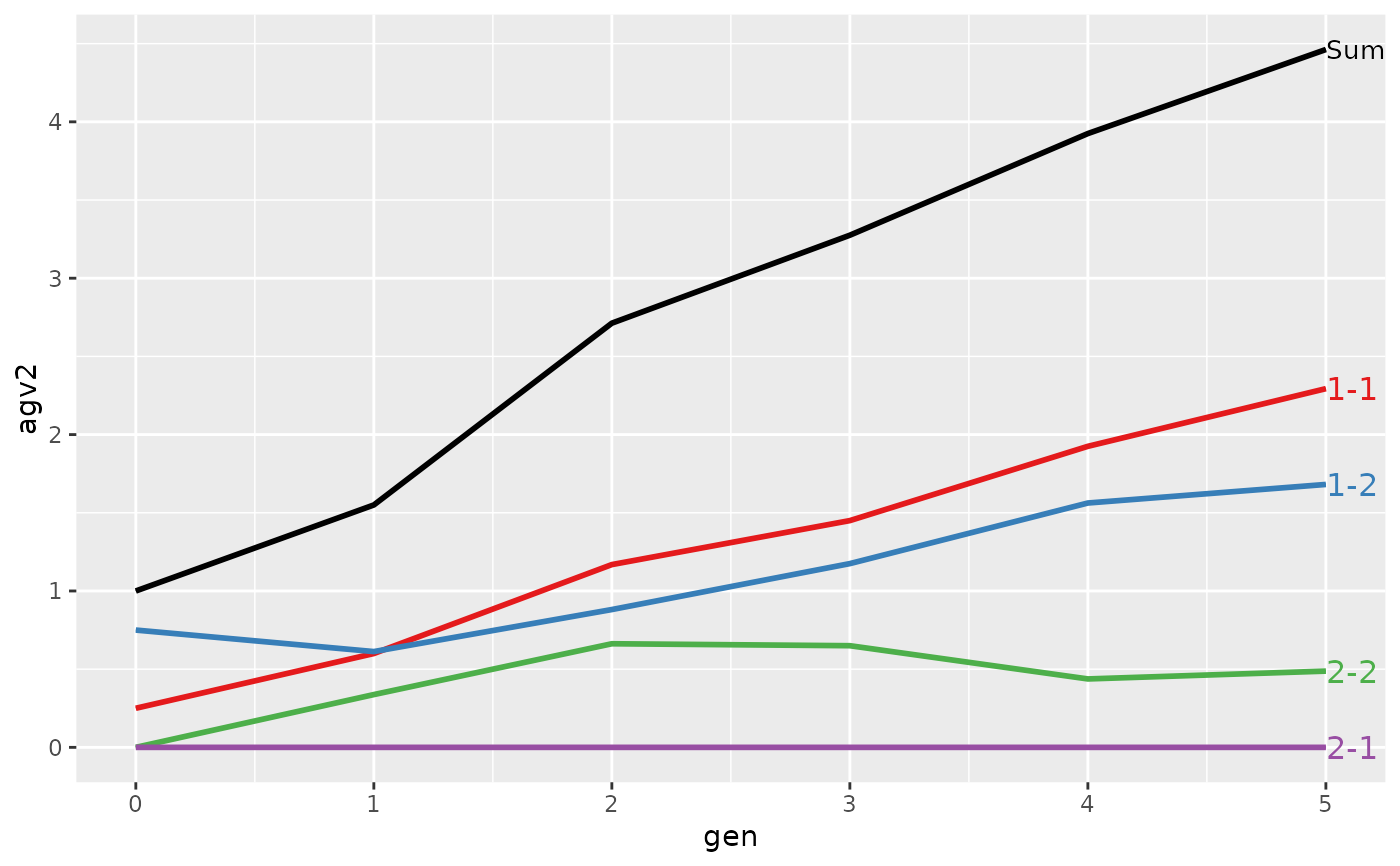
#> > ## Summarize and plot by generation (=trend)
#> > (ret <- summary(res, by="gen"))
#>
#>
#> Summary of partitions of breeding values
#> - paths: 2 (1, 2)
#> - traits: 2 (agv1, agv2)
#>
#> Trait: agv1
#>
#> gen N Sum 1 2
#> 1 0 8 1.0000 1.0000 0.0000
#> 2 1 8 1.4875 1.2125 0.2750
#> 3 2 8 1.8875 2.0500 -0.1625
#> 4 3 8 2.7500 2.6250 0.1250
#> 5 4 8 3.6125 3.4875 0.1250
#> 6 5 8 4.0625 3.9750 0.0875
#>
#> Trait: agv2
#>
#> gen N Sum 1 2
#> 1 0 8 1.0000 1.0000 0.0000
#> 2 1 8 1.5500 1.2125 0.3375
#> 3 2 8 2.7125 2.0500 0.6625
#> 4 3 8 3.2750 2.6250 0.6500
#> 5 4 8 3.9250 3.4875 0.4375
#> 6 5 8 4.4625 3.9750 0.4875
#>
#>
#> > plot(ret)
 #>
#> > ## Summarize and plot location specific trends
#> > (ret <- summary(res, by="loc.gen"))
#>
#>
#> Summary of partitions of breeding values
#> - paths: 2 (1, 2)
#> - traits: 2 (agv1, agv2)
#>
#> Trait: agv1
#>
#> loc.gen N Sum 1 2
#> 1 1-0 4 2.000 2.000 0.000
#> 2 1-1 4 2.425 2.425 0.000
#> 3 1-2 4 2.700 2.700 0.000
#> 4 1-3 4 3.250 3.250 0.000
#> 5 1-4 4 4.275 4.275 0.000
#> 6 1-5 4 4.600 4.600 0.000
#> 7 2-0 4 0.000 0.000 0.000
#> 8 2-1 4 0.550 0.000 0.550
#> 9 2-2 4 1.075 1.400 -0.325
#> 10 2-3 4 2.250 2.000 0.250
#> 11 2-4 4 2.950 2.700 0.250
#> 12 2-5 4 3.525 3.350 0.175
#>
#> Trait: agv2
#>
#> loc.gen N Sum 1 2
#> 1 1-0 4 2.000 2.000 0.000
#> 2 1-1 4 2.425 2.425 0.000
#> 3 1-2 4 2.700 2.700 0.000
#> 4 1-3 4 3.250 3.250 0.000
#> 5 1-4 4 4.275 4.275 0.000
#> 6 1-5 4 4.600 4.600 0.000
#> 7 2-0 4 0.000 0.000 0.000
#> 8 2-1 4 0.675 0.000 0.675
#> 9 2-2 4 2.725 1.400 1.325
#> 10 2-3 4 3.300 2.000 1.300
#> 11 2-4 4 3.575 2.700 0.875
#> 12 2-5 4 4.325 3.350 0.975
#>
#>
#> > plot(ret)
#>
#> > ## Summarize and plot location specific trends
#> > (ret <- summary(res, by="loc.gen"))
#>
#>
#> Summary of partitions of breeding values
#> - paths: 2 (1, 2)
#> - traits: 2 (agv1, agv2)
#>
#> Trait: agv1
#>
#> loc.gen N Sum 1 2
#> 1 1-0 4 2.000 2.000 0.000
#> 2 1-1 4 2.425 2.425 0.000
#> 3 1-2 4 2.700 2.700 0.000
#> 4 1-3 4 3.250 3.250 0.000
#> 5 1-4 4 4.275 4.275 0.000
#> 6 1-5 4 4.600 4.600 0.000
#> 7 2-0 4 0.000 0.000 0.000
#> 8 2-1 4 0.550 0.000 0.550
#> 9 2-2 4 1.075 1.400 -0.325
#> 10 2-3 4 2.250 2.000 0.250
#> 11 2-4 4 2.950 2.700 0.250
#> 12 2-5 4 3.525 3.350 0.175
#>
#> Trait: agv2
#>
#> loc.gen N Sum 1 2
#> 1 1-0 4 2.000 2.000 0.000
#> 2 1-1 4 2.425 2.425 0.000
#> 3 1-2 4 2.700 2.700 0.000
#> 4 1-3 4 3.250 3.250 0.000
#> 5 1-4 4 4.275 4.275 0.000
#> 6 1-5 4 4.600 4.600 0.000
#> 7 2-0 4 0.000 0.000 0.000
#> 8 2-1 4 0.675 0.000 0.675
#> 9 2-2 4 2.725 1.400 1.325
#> 10 2-3 4 3.300 2.000 1.300
#> 11 2-4 4 3.575 2.700 0.875
#> 12 2-5 4 4.325 3.350 0.975
#>
#>
#> > plot(ret)
 #>
#> > ## Summarize and plot location specific trends but only for location 1
#> > (ret <- summary(res, by="loc.gen", subset=res[[1]]$loc == 1))
#>
#>
#> Summary of partitions of breeding values
#> - paths: 2 (1, 2)
#> - traits: 2 (agv1, agv2)
#>
#> Trait: agv1
#>
#> loc.gen N Sum 1 2
#> 1 1-0 4 2.000 2.000 0
#> 2 1-1 4 2.425 2.425 0
#> 3 1-2 4 2.700 2.700 0
#> 4 1-3 4 3.250 3.250 0
#> 5 1-4 4 4.275 4.275 0
#> 6 1-5 4 4.600 4.600 0
#>
#> Trait: agv2
#>
#> loc.gen N Sum 1 2
#> 1 1-0 4 2.000 2.000 0
#> 2 1-1 4 2.425 2.425 0
#> 3 1-2 4 2.700 2.700 0
#> 4 1-3 4 3.250 3.250 0
#> 5 1-4 4 4.275 4.275 0
#> 6 1-5 4 4.600 4.600 0
#>
#>
#> > plot(ret)
#>
#> > ## Summarize and plot location specific trends but only for location 1
#> > (ret <- summary(res, by="loc.gen", subset=res[[1]]$loc == 1))
#>
#>
#> Summary of partitions of breeding values
#> - paths: 2 (1, 2)
#> - traits: 2 (agv1, agv2)
#>
#> Trait: agv1
#>
#> loc.gen N Sum 1 2
#> 1 1-0 4 2.000 2.000 0
#> 2 1-1 4 2.425 2.425 0
#> 3 1-2 4 2.700 2.700 0
#> 4 1-3 4 3.250 3.250 0
#> 5 1-4 4 4.275 4.275 0
#> 6 1-5 4 4.600 4.600 0
#>
#> Trait: agv2
#>
#> loc.gen N Sum 1 2
#> 1 1-0 4 2.000 2.000 0
#> 2 1-1 4 2.425 2.425 0
#> 3 1-2 4 2.700 2.700 0
#> 4 1-3 4 3.250 3.250 0
#> 5 1-4 4 4.275 4.275 0
#> 6 1-5 4 4.600 4.600 0
#>
#>
#> > plot(ret)
 #>
#> > ## Summarize and plot location specific trends but only for location 2
#> > (ret <- summary(res, by="loc.gen", subset=res[[1]]$loc == 2))
#>
#>
#> Summary of partitions of breeding values
#> - paths: 2 (1, 2)
#> - traits: 2 (agv1, agv2)
#>
#> Trait: agv1
#>
#> loc.gen N Sum 1 2
#> 1 2-0 4 0.000 0.00 0.000
#> 2 2-1 4 0.550 0.00 0.550
#> 3 2-2 4 1.075 1.40 -0.325
#> 4 2-3 4 2.250 2.00 0.250
#> 5 2-4 4 2.950 2.70 0.250
#> 6 2-5 4 3.525 3.35 0.175
#>
#> Trait: agv2
#>
#> loc.gen N Sum 1 2
#> 1 2-0 4 0.000 0.00 0.000
#> 2 2-1 4 0.675 0.00 0.675
#> 3 2-2 4 2.725 1.40 1.325
#> 4 2-3 4 3.300 2.00 1.300
#> 5 2-4 4 3.575 2.70 0.875
#> 6 2-5 4 4.325 3.35 0.975
#>
#>
#> > plot(ret)
#>
#> > ## Summarize and plot location specific trends but only for location 2
#> > (ret <- summary(res, by="loc.gen", subset=res[[1]]$loc == 2))
#>
#>
#> Summary of partitions of breeding values
#> - paths: 2 (1, 2)
#> - traits: 2 (agv1, agv2)
#>
#> Trait: agv1
#>
#> loc.gen N Sum 1 2
#> 1 2-0 4 0.000 0.00 0.000
#> 2 2-1 4 0.550 0.00 0.550
#> 3 2-2 4 1.075 1.40 -0.325
#> 4 2-3 4 2.250 2.00 0.250
#> 5 2-4 4 2.950 2.70 0.250
#> 6 2-5 4 3.525 3.35 0.175
#>
#> Trait: agv2
#>
#> loc.gen N Sum 1 2
#> 1 2-0 4 0.000 0.00 0.000
#> 2 2-1 4 0.675 0.00 0.675
#> 3 2-2 4 2.725 1.40 1.325
#> 4 2-3 4 3.300 2.00 1.300
#> 5 2-4 4 3.575 2.70 0.875
#> 6 2-5 4 4.325 3.35 0.975
#>
#>
#> > plot(ret)
 #>
#> > ## Compute partitions by location and sex
#> > ped$loc.sex <- with(ped, paste(loc, sex, sep="-"))
#>
#> > (res <- AlphaPart(x=ped, colPath="loc.sex", colBV=c("agv1", "agv2")))
#>
#> Size:
#> - individuals: 48
#> - traits: 2 (agv1, agv2)
#> - paths: 4 (1-1, 1-2, 2-1, 2-2)
#> - unknown (missing) values:
#> agv1 agv2
#> 0 0
#>
#>
#> Partitions of breeding values
#> - individuals: 48
#> - paths: 4 (1-1, 1-2, 2-1, 2-2)
#> - traits: 2 (agv1, agv2)
#>
#> Trait: agv1
#>
#> id fid mid loc gen sex loc.gen loc.sex agv1 agv1_pa agv1_w agv1_1-1 agv1_1-2 agv1_2-1 agv1_2-2
#> 1 01 <NA> <NA> 1 0 2 1-0 1-2 2 1 1 0 2 0 0
#> 2 02 <NA> <NA> 1 0 1 1-0 1-1 2 1 1 2 0 0 0
#> 3 03 <NA> <NA> 1 0 2 1-0 1-2 2 1 1 0 2 0 0
#> 4 04 <NA> <NA> 1 0 2 1-0 1-2 2 1 1 0 2 0 0
#> 5 05 <NA> <NA> 2 0 2 2-0 2-2 0 1 -1 0 0 0 0
#> 6 06 <NA> <NA> 2 0 1 2-0 2-1 0 1 -1 0 0 0 0
#> ...
#> id fid mid loc gen sex loc.gen loc.sex agv1 agv1_pa agv1_w agv1_1-1 agv1_1-2 agv1_2-1 agv1_2-2
#> 43 53 44 43 1 5 2 1-5 1-2 5.3 4.15 1.15 2.3250 2.9750 0 0.00
#> 44 54 44 43 1 5 2 1-5 1-2 4.2 4.15 0.05 2.3250 1.8750 0 0.00
#> 45 55 44 45 2 5 2 2-5 2-2 4.1 3.15 0.95 2.2625 1.0875 0 0.75
#> 46 56 44 46 2 5 2 2-5 2-2 2.7 3.20 -0.50 2.2625 1.0875 0 -0.65
#> 47 57 44 47 2 5 2 2-5 2-2 3.5 3.20 0.30 2.2625 1.0875 0 0.15
#> 48 58 44 48 2 5 2 2-5 2-2 3.8 4.35 -0.55 2.2625 1.0875 0 0.45
#>
#> Trait: agv2
#>
#> id fid mid loc gen sex loc.gen loc.sex agv2 agv2_pa agv2_w agv2_1-1 agv2_1-2 agv2_2-1 agv2_2-2
#> 1 01 <NA> <NA> 1 0 2 1-0 1-2 2 1 1 0 2 0 0
#> 2 02 <NA> <NA> 1 0 1 1-0 1-1 2 1 1 2 0 0 0
#> 3 03 <NA> <NA> 1 0 2 1-0 1-2 2 1 1 0 2 0 0
#> 4 04 <NA> <NA> 1 0 2 1-0 1-2 2 1 1 0 2 0 0
#> 5 05 <NA> <NA> 2 0 2 2-0 2-2 0 1 -1 0 0 0 0
#> 6 06 <NA> <NA> 2 0 1 2-0 2-1 0 1 -1 0 0 0 0
#> ...
#> id fid mid loc gen sex loc.gen loc.sex agv2 agv2_pa agv2_w agv2_1-1 agv2_1-2 agv2_2-1 agv2_2-2
#> 43 53 44 43 1 5 2 1-5 1-2 5.3 4.15 1.15 2.3250 2.9750 0 0.00
#> 44 54 44 43 1 5 2 1-5 1-2 4.2 4.15 0.05 2.3250 1.8750 0 0.00
#> 45 55 44 45 2 5 2 2-5 2-2 3.7 3.65 0.05 2.2625 1.0875 0 0.35
#> 46 56 44 46 2 5 2 2-5 2-2 5.2 4.00 1.20 2.2625 1.0875 0 1.85
#> 47 57 44 47 2 5 2 2-5 2-2 4.1 3.90 0.20 2.2625 1.0875 0 0.75
#> 48 58 44 48 2 5 2 2-5 2-2 4.3 3.60 0.70 2.2625 1.0875 0 0.95
#>
#>
#> > ## Summarize and plot by generation (=trend)
#> > (ret <- summary(res, by="gen"))
#>
#>
#> Summary of partitions of breeding values
#> - paths: 4 (1-1, 1-2, 2-1, 2-2)
#> - traits: 2 (agv1, agv2)
#>
#> Trait: agv1
#>
#> gen N Sum 1-1 1-2 2-1 2-2
#> 1 0 8 1.0000 0.25000 0.75000 0 0.0000
#> 2 1 8 1.4875 0.60000 0.61250 0 0.2750
#> 3 2 8 1.8875 1.16875 0.88125 0 -0.1625
#> 4 3 8 2.7500 1.45000 1.17500 0 0.1250
#> 5 4 8 3.6125 1.92500 1.56250 0 0.1250
#> 6 5 8 4.0625 2.29375 1.68125 0 0.0875
#>
#> Trait: agv2
#>
#> gen N Sum 1-1 1-2 2-1 2-2
#> 1 0 8 1.0000 0.25000 0.75000 0 0.0000
#> 2 1 8 1.5500 0.60000 0.61250 0 0.3375
#> 3 2 8 2.7125 1.16875 0.88125 0 0.6625
#> 4 3 8 3.2750 1.45000 1.17500 0 0.6500
#> 5 4 8 3.9250 1.92500 1.56250 0 0.4375
#> 6 5 8 4.4625 2.29375 1.68125 0 0.4875
#>
#>
#> > plot(ret)
#>
#> > ## Compute partitions by location and sex
#> > ped$loc.sex <- with(ped, paste(loc, sex, sep="-"))
#>
#> > (res <- AlphaPart(x=ped, colPath="loc.sex", colBV=c("agv1", "agv2")))
#>
#> Size:
#> - individuals: 48
#> - traits: 2 (agv1, agv2)
#> - paths: 4 (1-1, 1-2, 2-1, 2-2)
#> - unknown (missing) values:
#> agv1 agv2
#> 0 0
#>
#>
#> Partitions of breeding values
#> - individuals: 48
#> - paths: 4 (1-1, 1-2, 2-1, 2-2)
#> - traits: 2 (agv1, agv2)
#>
#> Trait: agv1
#>
#> id fid mid loc gen sex loc.gen loc.sex agv1 agv1_pa agv1_w agv1_1-1 agv1_1-2 agv1_2-1 agv1_2-2
#> 1 01 <NA> <NA> 1 0 2 1-0 1-2 2 1 1 0 2 0 0
#> 2 02 <NA> <NA> 1 0 1 1-0 1-1 2 1 1 2 0 0 0
#> 3 03 <NA> <NA> 1 0 2 1-0 1-2 2 1 1 0 2 0 0
#> 4 04 <NA> <NA> 1 0 2 1-0 1-2 2 1 1 0 2 0 0
#> 5 05 <NA> <NA> 2 0 2 2-0 2-2 0 1 -1 0 0 0 0
#> 6 06 <NA> <NA> 2 0 1 2-0 2-1 0 1 -1 0 0 0 0
#> ...
#> id fid mid loc gen sex loc.gen loc.sex agv1 agv1_pa agv1_w agv1_1-1 agv1_1-2 agv1_2-1 agv1_2-2
#> 43 53 44 43 1 5 2 1-5 1-2 5.3 4.15 1.15 2.3250 2.9750 0 0.00
#> 44 54 44 43 1 5 2 1-5 1-2 4.2 4.15 0.05 2.3250 1.8750 0 0.00
#> 45 55 44 45 2 5 2 2-5 2-2 4.1 3.15 0.95 2.2625 1.0875 0 0.75
#> 46 56 44 46 2 5 2 2-5 2-2 2.7 3.20 -0.50 2.2625 1.0875 0 -0.65
#> 47 57 44 47 2 5 2 2-5 2-2 3.5 3.20 0.30 2.2625 1.0875 0 0.15
#> 48 58 44 48 2 5 2 2-5 2-2 3.8 4.35 -0.55 2.2625 1.0875 0 0.45
#>
#> Trait: agv2
#>
#> id fid mid loc gen sex loc.gen loc.sex agv2 agv2_pa agv2_w agv2_1-1 agv2_1-2 agv2_2-1 agv2_2-2
#> 1 01 <NA> <NA> 1 0 2 1-0 1-2 2 1 1 0 2 0 0
#> 2 02 <NA> <NA> 1 0 1 1-0 1-1 2 1 1 2 0 0 0
#> 3 03 <NA> <NA> 1 0 2 1-0 1-2 2 1 1 0 2 0 0
#> 4 04 <NA> <NA> 1 0 2 1-0 1-2 2 1 1 0 2 0 0
#> 5 05 <NA> <NA> 2 0 2 2-0 2-2 0 1 -1 0 0 0 0
#> 6 06 <NA> <NA> 2 0 1 2-0 2-1 0 1 -1 0 0 0 0
#> ...
#> id fid mid loc gen sex loc.gen loc.sex agv2 agv2_pa agv2_w agv2_1-1 agv2_1-2 agv2_2-1 agv2_2-2
#> 43 53 44 43 1 5 2 1-5 1-2 5.3 4.15 1.15 2.3250 2.9750 0 0.00
#> 44 54 44 43 1 5 2 1-5 1-2 4.2 4.15 0.05 2.3250 1.8750 0 0.00
#> 45 55 44 45 2 5 2 2-5 2-2 3.7 3.65 0.05 2.2625 1.0875 0 0.35
#> 46 56 44 46 2 5 2 2-5 2-2 5.2 4.00 1.20 2.2625 1.0875 0 1.85
#> 47 57 44 47 2 5 2 2-5 2-2 4.1 3.90 0.20 2.2625 1.0875 0 0.75
#> 48 58 44 48 2 5 2 2-5 2-2 4.3 3.60 0.70 2.2625 1.0875 0 0.95
#>
#>
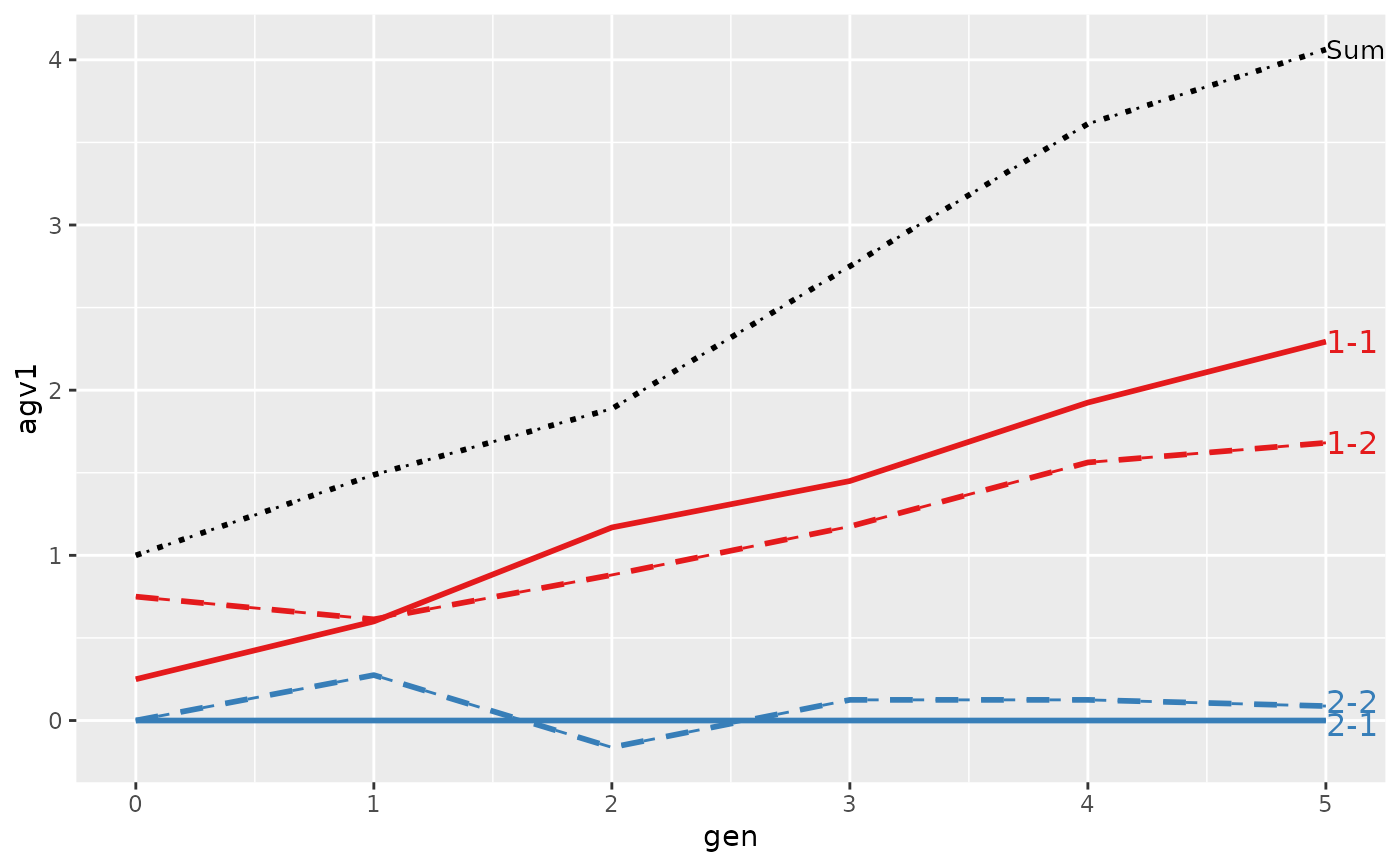
#> > ## Summarize and plot by generation (=trend)
#> > (ret <- summary(res, by="gen"))
#>
#>
#> Summary of partitions of breeding values
#> - paths: 4 (1-1, 1-2, 2-1, 2-2)
#> - traits: 2 (agv1, agv2)
#>
#> Trait: agv1
#>
#> gen N Sum 1-1 1-2 2-1 2-2
#> 1 0 8 1.0000 0.25000 0.75000 0 0.0000
#> 2 1 8 1.4875 0.60000 0.61250 0 0.2750
#> 3 2 8 1.8875 1.16875 0.88125 0 -0.1625
#> 4 3 8 2.7500 1.45000 1.17500 0 0.1250
#> 5 4 8 3.6125 1.92500 1.56250 0 0.1250
#> 6 5 8 4.0625 2.29375 1.68125 0 0.0875
#>
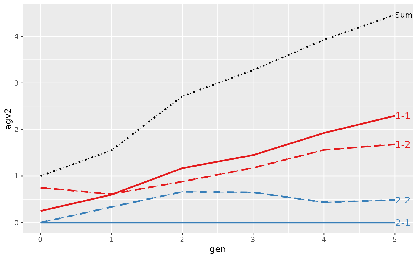
#> Trait: agv2
#>
#> gen N Sum 1-1 1-2 2-1 2-2
#> 1 0 8 1.0000 0.25000 0.75000 0 0.0000
#> 2 1 8 1.5500 0.60000 0.61250 0 0.3375
#> 3 2 8 2.7125 1.16875 0.88125 0 0.6625
#> 4 3 8 3.2750 1.45000 1.17500 0 0.6500
#> 5 4 8 3.9250 1.92500 1.56250 0 0.4375
#> 6 5 8 4.4625 2.29375 1.68125 0 0.4875
#>
#>
#> > plot(ret)
 #>
#> > plot(ret, lineTypeList=list("-1"=1, "-2"=2, def=3))
#>
#> > plot(ret, lineTypeList=list("-1"=1, "-2"=2, def=3))
 #>
#> > ## Summarize and plot location specific trends
#> > (ret <- summary(res, by="loc.gen"))
#>
#>
#> Summary of partitions of breeding values
#> - paths: 4 (1-1, 1-2, 2-1, 2-2)
#> - traits: 2 (agv1, agv2)
#>
#> Trait: agv1
#>
#> loc.gen N Sum 1-1 1-2 2-1 2-2
#> 1 1-0 4 2.000 0.5000 1.5000 0 0.000
#> 2 1-1 4 2.425 1.2000 1.2250 0 0.000
#> 3 1-2 4 2.700 1.4375 1.2625 0 0.000
#> 4 1-3 4 3.250 1.6750 1.5750 0 0.000
#> 5 1-4 4 4.275 2.1000 2.1750 0 0.000
#> 6 1-5 4 4.600 2.3250 2.2750 0 0.000
#> 7 2-0 4 0.000 0.0000 0.0000 0 0.000
#> 8 2-1 4 0.550 0.0000 0.0000 0 0.550
#> 9 2-2 4 1.075 0.9000 0.5000 0 -0.325
#> 10 2-3 4 2.250 1.2250 0.7750 0 0.250
#> 11 2-4 4 2.950 1.7500 0.9500 0 0.250
#> 12 2-5 4 3.525 2.2625 1.0875 0 0.175
#>
#> Trait: agv2
#>
#> loc.gen N Sum 1-1 1-2 2-1 2-2
#> 1 1-0 4 2.000 0.5000 1.5000 0 0.000
#> 2 1-1 4 2.425 1.2000 1.2250 0 0.000
#> 3 1-2 4 2.700 1.4375 1.2625 0 0.000
#> 4 1-3 4 3.250 1.6750 1.5750 0 0.000
#> 5 1-4 4 4.275 2.1000 2.1750 0 0.000
#> 6 1-5 4 4.600 2.3250 2.2750 0 0.000
#> 7 2-0 4 0.000 0.0000 0.0000 0 0.000
#> 8 2-1 4 0.675 0.0000 0.0000 0 0.675
#> 9 2-2 4 2.725 0.9000 0.5000 0 1.325
#> 10 2-3 4 3.300 1.2250 0.7750 0 1.300
#> 11 2-4 4 3.575 1.7500 0.9500 0 0.875
#> 12 2-5 4 4.325 2.2625 1.0875 0 0.975
#>
#>
#> > plot(ret, lineTypeList=list("-1"=1, "-2"=2, def=3))
#>
#> > ## Summarize and plot location specific trends
#> > (ret <- summary(res, by="loc.gen"))
#>
#>
#> Summary of partitions of breeding values
#> - paths: 4 (1-1, 1-2, 2-1, 2-2)
#> - traits: 2 (agv1, agv2)
#>
#> Trait: agv1
#>
#> loc.gen N Sum 1-1 1-2 2-1 2-2
#> 1 1-0 4 2.000 0.5000 1.5000 0 0.000
#> 2 1-1 4 2.425 1.2000 1.2250 0 0.000
#> 3 1-2 4 2.700 1.4375 1.2625 0 0.000
#> 4 1-3 4 3.250 1.6750 1.5750 0 0.000
#> 5 1-4 4 4.275 2.1000 2.1750 0 0.000
#> 6 1-5 4 4.600 2.3250 2.2750 0 0.000
#> 7 2-0 4 0.000 0.0000 0.0000 0 0.000
#> 8 2-1 4 0.550 0.0000 0.0000 0 0.550
#> 9 2-2 4 1.075 0.9000 0.5000 0 -0.325
#> 10 2-3 4 2.250 1.2250 0.7750 0 0.250
#> 11 2-4 4 2.950 1.7500 0.9500 0 0.250
#> 12 2-5 4 3.525 2.2625 1.0875 0 0.175
#>
#> Trait: agv2
#>
#> loc.gen N Sum 1-1 1-2 2-1 2-2
#> 1 1-0 4 2.000 0.5000 1.5000 0 0.000
#> 2 1-1 4 2.425 1.2000 1.2250 0 0.000
#> 3 1-2 4 2.700 1.4375 1.2625 0 0.000
#> 4 1-3 4 3.250 1.6750 1.5750 0 0.000
#> 5 1-4 4 4.275 2.1000 2.1750 0 0.000
#> 6 1-5 4 4.600 2.3250 2.2750 0 0.000
#> 7 2-0 4 0.000 0.0000 0.0000 0 0.000
#> 8 2-1 4 0.675 0.0000 0.0000 0 0.675
#> 9 2-2 4 2.725 0.9000 0.5000 0 1.325
#> 10 2-3 4 3.300 1.2250 0.7750 0 1.300
#> 11 2-4 4 3.575 1.7500 0.9500 0 0.875
#> 12 2-5 4 4.325 2.2625 1.0875 0 0.975
#>
#>
#> > plot(ret, lineTypeList=list("-1"=1, "-2"=2, def=3))
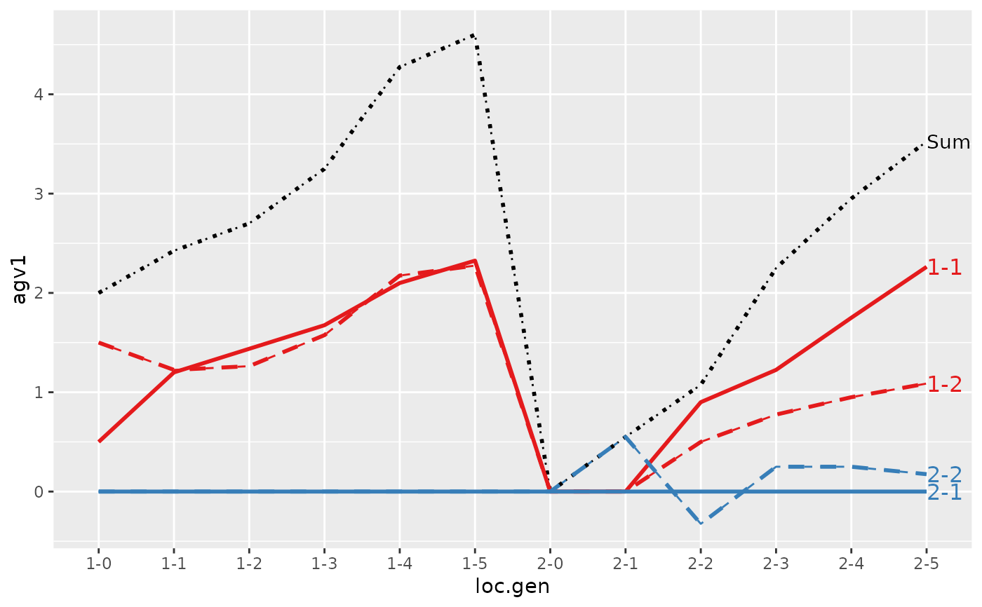
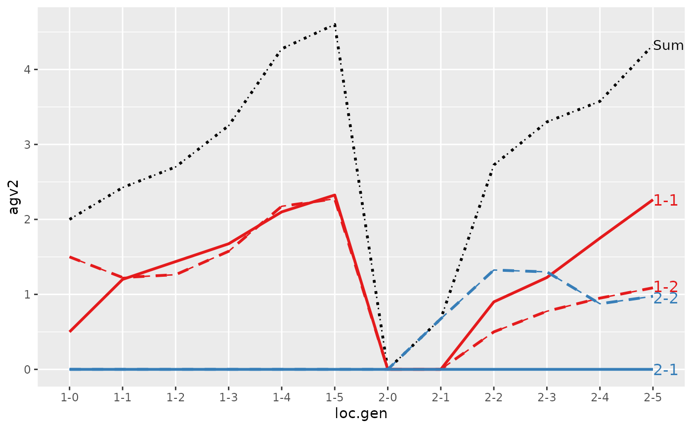 #>
#> > ## Summarize and plot location specific trends but only for location 1
#> > (ret <- summary(res, by="loc.gen", subset=res[[1]]$loc == 1))
#>
#>
#> Summary of partitions of breeding values
#> - paths: 4 (1-1, 1-2, 2-1, 2-2)
#> - traits: 2 (agv1, agv2)
#>
#> Trait: agv1
#>
#> loc.gen N Sum 1-1 1-2 2-1 2-2
#> 1 1-0 4 2.000 0.5000 1.5000 0 0
#> 2 1-1 4 2.425 1.2000 1.2250 0 0
#> 3 1-2 4 2.700 1.4375 1.2625 0 0
#> 4 1-3 4 3.250 1.6750 1.5750 0 0
#> 5 1-4 4 4.275 2.1000 2.1750 0 0
#> 6 1-5 4 4.600 2.3250 2.2750 0 0
#>
#> Trait: agv2
#>
#> loc.gen N Sum 1-1 1-2 2-1 2-2
#> 1 1-0 4 2.000 0.5000 1.5000 0 0
#> 2 1-1 4 2.425 1.2000 1.2250 0 0
#> 3 1-2 4 2.700 1.4375 1.2625 0 0
#> 4 1-3 4 3.250 1.6750 1.5750 0 0
#> 5 1-4 4 4.275 2.1000 2.1750 0 0
#> 6 1-5 4 4.600 2.3250 2.2750 0 0
#>
#>
#> > plot(ret)
#>
#> > ## Summarize and plot location specific trends but only for location 1
#> > (ret <- summary(res, by="loc.gen", subset=res[[1]]$loc == 1))
#>
#>
#> Summary of partitions of breeding values
#> - paths: 4 (1-1, 1-2, 2-1, 2-2)
#> - traits: 2 (agv1, agv2)
#>
#> Trait: agv1
#>
#> loc.gen N Sum 1-1 1-2 2-1 2-2
#> 1 1-0 4 2.000 0.5000 1.5000 0 0
#> 2 1-1 4 2.425 1.2000 1.2250 0 0
#> 3 1-2 4 2.700 1.4375 1.2625 0 0
#> 4 1-3 4 3.250 1.6750 1.5750 0 0
#> 5 1-4 4 4.275 2.1000 2.1750 0 0
#> 6 1-5 4 4.600 2.3250 2.2750 0 0
#>
#> Trait: agv2
#>
#> loc.gen N Sum 1-1 1-2 2-1 2-2
#> 1 1-0 4 2.000 0.5000 1.5000 0 0
#> 2 1-1 4 2.425 1.2000 1.2250 0 0
#> 3 1-2 4 2.700 1.4375 1.2625 0 0
#> 4 1-3 4 3.250 1.6750 1.5750 0 0
#> 5 1-4 4 4.275 2.1000 2.1750 0 0
#> 6 1-5 4 4.600 2.3250 2.2750 0 0
#>
#>
#> > plot(ret)

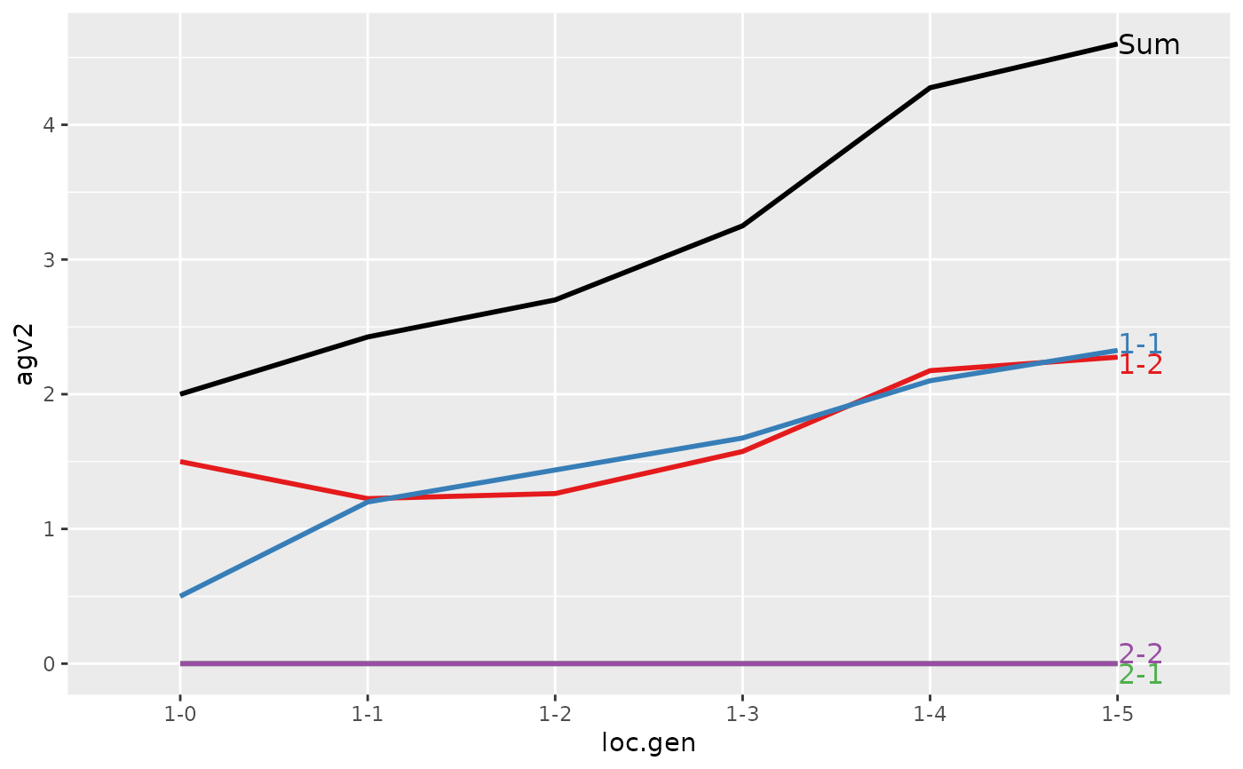 #>
#> > ## Summarize and plot location specific trends but only for location 2
#> > (ret <- summary(res, by="loc.gen", subset=res[[1]]$loc == 2))
#>
#>
#> Summary of partitions of breeding values
#> - paths: 4 (1-1, 1-2, 2-1, 2-2)
#> - traits: 2 (agv1, agv2)
#>
#> Trait: agv1
#>
#> loc.gen N Sum 1-1 1-2 2-1 2-2
#> 1 2-0 4 0.000 0.0000 0.0000 0 0.000
#> 2 2-1 4 0.550 0.0000 0.0000 0 0.550
#> 3 2-2 4 1.075 0.9000 0.5000 0 -0.325
#> 4 2-3 4 2.250 1.2250 0.7750 0 0.250
#> 5 2-4 4 2.950 1.7500 0.9500 0 0.250
#> 6 2-5 4 3.525 2.2625 1.0875 0 0.175
#>
#> Trait: agv2
#>
#> loc.gen N Sum 1-1 1-2 2-1 2-2
#> 1 2-0 4 0.000 0.0000 0.0000 0 0.000
#> 2 2-1 4 0.675 0.0000 0.0000 0 0.675
#> 3 2-2 4 2.725 0.9000 0.5000 0 1.325
#> 4 2-3 4 3.300 1.2250 0.7750 0 1.300
#> 5 2-4 4 3.575 1.7500 0.9500 0 0.875
#> 6 2-5 4 4.325 2.2625 1.0875 0 0.975
#>
#>
#> > plot(ret)
#>
#> > ## Summarize and plot location specific trends but only for location 2
#> > (ret <- summary(res, by="loc.gen", subset=res[[1]]$loc == 2))
#>
#>
#> Summary of partitions of breeding values
#> - paths: 4 (1-1, 1-2, 2-1, 2-2)
#> - traits: 2 (agv1, agv2)
#>
#> Trait: agv1
#>
#> loc.gen N Sum 1-1 1-2 2-1 2-2
#> 1 2-0 4 0.000 0.0000 0.0000 0 0.000
#> 2 2-1 4 0.550 0.0000 0.0000 0 0.550
#> 3 2-2 4 1.075 0.9000 0.5000 0 -0.325
#> 4 2-3 4 2.250 1.2250 0.7750 0 0.250
#> 5 2-4 4 2.950 1.7500 0.9500 0 0.250
#> 6 2-5 4 3.525 2.2625 1.0875 0 0.175
#>
#> Trait: agv2
#>
#> loc.gen N Sum 1-1 1-2 2-1 2-2
#> 1 2-0 4 0.000 0.0000 0.0000 0 0.000
#> 2 2-1 4 0.675 0.0000 0.0000 0 0.675
#> 3 2-2 4 2.725 0.9000 0.5000 0 1.325
#> 4 2-3 4 3.300 1.2250 0.7750 0 1.300
#> 5 2-4 4 3.575 1.7500 0.9500 0 0.875
#> 6 2-5 4 4.325 2.2625 1.0875 0 0.975
#>
#>
#> > plot(ret)
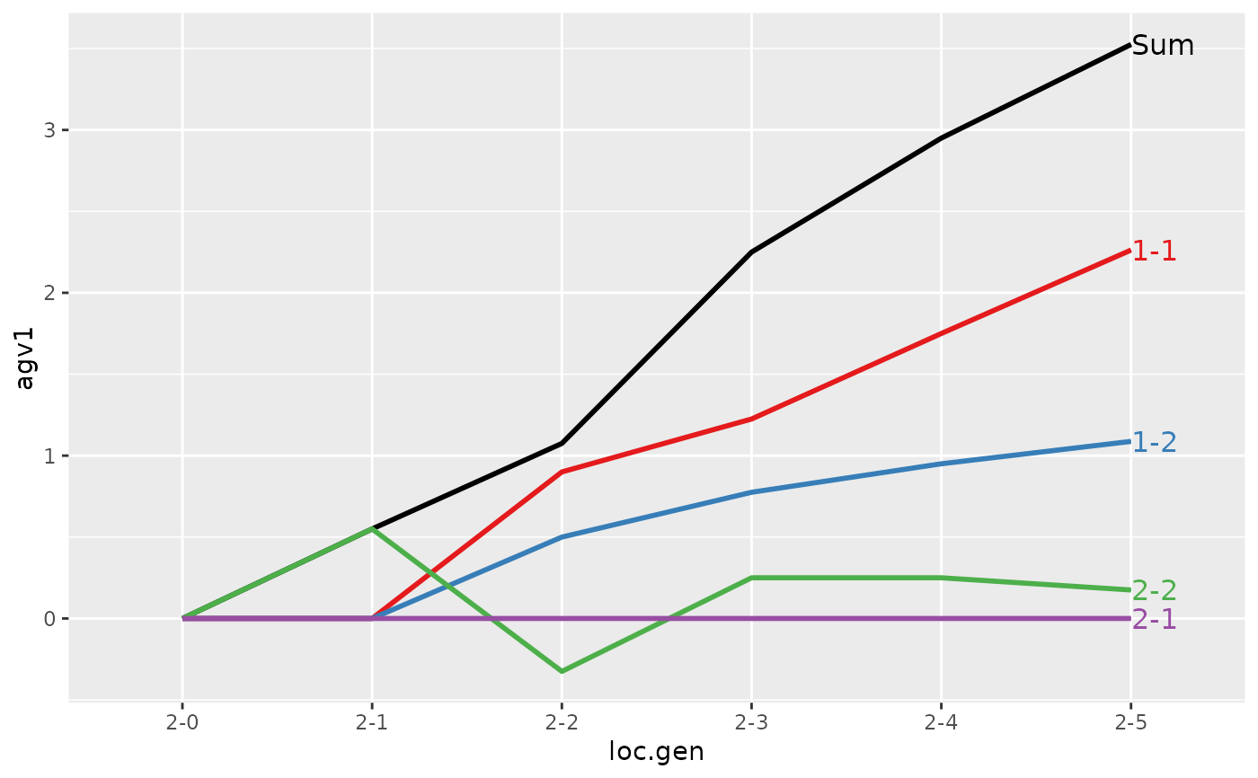
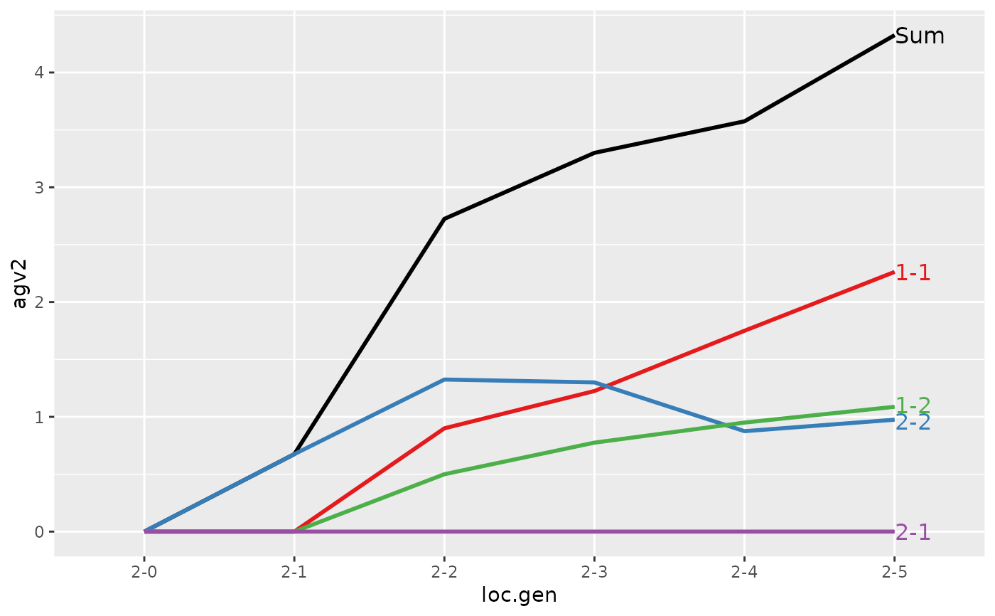 #>
#> > ###-----------------------------------------------------------------------------
#> > ### demo_stohastic.R ends here
# }
#>
#> > ###-----------------------------------------------------------------------------
#> > ### demo_stohastic.R ends here
# }